The Monte Carlo method is a computational algorithm that relies on repeated random sampling to obtain numerical results. It is often used to solve problems that are deterministic in nature but are difficult to solve analytically. The method is named after the Monte Carlo Casino in Monaco, where random sampling is a common practice.
First let’s import the necessary libraries,
import random, math
import matplotlib.pyplot as plt
from shapely.geometry import Point, Polygon
1 - Area of an Irregular Shape
Now let’s define our shape,
coords = [(1, 1), (10, 95), (40, 70), (50, 50),(30,20)]
map = Polygon(coords) # will use later

# x, y = zip(*coords)
# alternatively, we can find the value of x and y using list comprehension as follows:
x = [coord[0] for coord in coords]
y = [coord[1] for coord in coords]

plt.plot(x + [x[0],], y + [y[0],], color="red")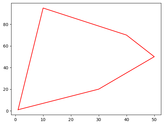
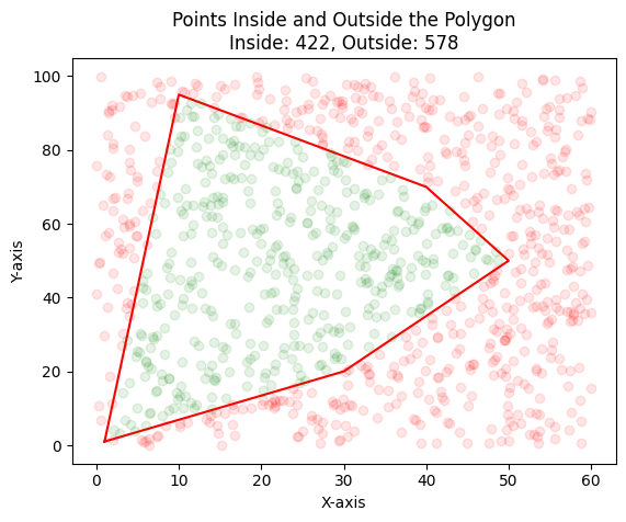
And finally the algorithm to calculate the area of the shape,
x_point = []
y_point = []

inside = 0
outside = 0

for _ in range(1000):
    x_rand = random.uniform(0, 60)
    y_rand = random.uniform(0, 100)
    point = Point(x_rand, y_rand)
    if map.contains(point):
        inside += 1
        x_point.append(x_rand)
        y_point.append(y_rand)
    else:
        outside += 1
        plt.plot(x_rand, y_rand, 'ro', alpha=0.1)

plt.plot(x + [x[0],], y + [y[0],], color="red")
plt.plot(x_point, y_point, 'go', alpha=0.1)
plt.title(f'Points Inside and Outside the Polygon\nInside: {inside}, Outside: {outside}')
plt.xlabel('X-axis')
plt.ylabel('Y-axis')

area_map = map.area
predicted_area = (inside / (inside + outside)) * (60 * 100)
print(f"Predicted Area: {predicted_area}, Actual Area: {area_map}")
Predicted Area: 2532.0, Actual Area: 2502.5
2 - A Gambling Game
In this game, binary coin are toasted, with two variable, cumulative heads and cumulative tails. You win if the difference between the two is 3, or the game continues!
class GamblingGame:
    def __init__(self):
        self.serial = 0
        self.cum_head = 0
        self.cum_tail = 0

    def run(self):
        while True:
            self.serial += 1
            random_num = random.randint(0, 1)
            if random_num == 0:
                self.cum_head += 1
            else:
                self.cum_tail += 1
            diff = abs(self.cum_head - self.cum_tail)
            if diff == 3:
                return 8 - self.serial


if __name__ == "__main__":
    run = 50
    total_rev = 0

    while run > 0:
        game = GamblingGame()
        total_rev += game.run()
        run -= 1

    print("Total rev : ", total_rev)
Total rev : -48
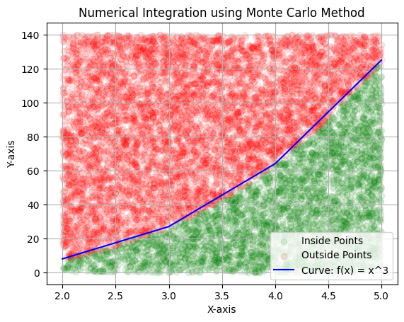
3 - Numerical Integration
Let’s integrate using the Monte Carlo method.
def fun(x):
    return x**3

class NumericalIntegration:
    def __init__(self, range_x_in, range_x_out, range_y_in, range_y_out, iteration=50):
        self.inside = 0
        self.outside = 0
        self.iteration = iteration
        self.range_x_in = range_x_in
        self.range_x_out = range_x_out
        self.range_y_in = range_y_in
        self.range_y_out = range_y_out
        self.points_inside = []
        self.points_outside = []

    def run(self):
        iteration = self.iteration
        while iteration > 0:
            random_num_x = random.uniform(self.range_x_in, self.range_x_out)
            random_num_y = random.uniform(self.range_y_in, self.range_y_out)

            y_real_value = fun(random_num_x)
            if random_num_y <= y_real_value:
                self.inside += 1
                self.points_inside.append((random_num_x, random_num_y))
            else:
                self.outside += 1
                self.points_outside.append((random_num_x, random_num_y))

            iteration -= 1

    def area_approximate(self):
        self.run()

        rectangle_area = (self.range_x_out - self.range_x_in) * (self.range_y_out - self.range_y_in)
        return (self.inside / (self.inside + self.outside) * rectangle_area)

    def plot(self):
        x_inside, y_inside = zip(*self.points_inside)
        x_outside, y_outside = zip(*self.points_outside)

        plt.scatter(x_inside, y_inside, color='green', alpha=0.1, label='Inside Points')
        plt.scatter(x_outside, y_outside, color='red', alpha=0.1, label='Outside Points')

        x_curve = [x for x in range(self.range_x_in, self.range_x_out + 1)]
        y_curve = [fun(x) for x in x_curve]
        plt.plot(x_curve, y_curve, color='blue', label='Curve: f(x) = x^3')

        plt.title('Numerical Integration using Monte Carlo Method')
        plt.xlabel('X-axis')
        plt.ylabel('Y-axis')
        plt.legend()
        plt.grid()
        plt.show()

areaFinder = NumericalIntegration(2, 5, 0, 140, 10000)
print(areaFinder.area_approximate())
areaFinder.plot()
152.208
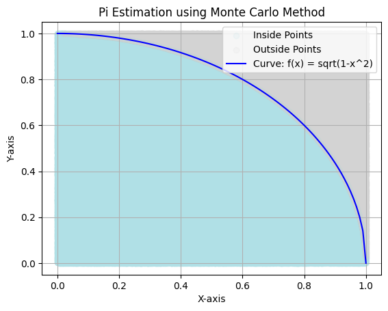
4 - Estimating Pi
def fun(x):
    return math.sqrt(1-x*x)

class PiEstimation:
    def __init__(self, range_x_in, range_x_out, range_y_in, range_y_out, iteration=50):
        self.inside = 0
        self.outside = 0
        self.iteration = iteration
        self.range_x_in = range_x_in
        self.range_x_out = range_x_out
        self.range_y_in = range_y_in
        self.range_y_out = range_y_out
        self.points_inside = []
        self.points_outside = []

    def run(self):
        iteration = self.iteration
        while iteration > 0:
            random_num_x = random.random()
            random_num_y = random.random()

            y_real_value = fun(random_num_x)
            if random_num_y <= y_real_value:
                self.inside += 1
                self.points_inside.append((random_num_x, random_num_y))

            else:
                self.outside += 1
                self.points_outside.append((random_num_x, random_num_y))


            iteration -= 1

    def area_approximate(self):
        self.run()
        return (self.inside / (self.inside + self.outside) * 4)

    def plot(self):
        x_inside, y_inside = zip(*self.points_inside)
        x_outside, y_outside = zip(*self.points_outside)

        plt.scatter(x_inside, y_inside, color='powderblue', alpha=0.1, label='Inside Points')
        plt.scatter(x_outside, y_outside, color='lightgray', alpha=0.1, label='Outside Points')

        x_curve = [x/100 for x in range(0, 101)]
        y_curve = [fun(x) for x in x_curve]
        plt.plot(x_curve, y_curve, color='blue', label='Curve: f(x) = sqrt(1-x^2)')

        plt.title('Pi Estimation using Monte Carlo Method')
        plt.xlabel('X-axis')
        plt.ylabel('Y-axis')
        plt.legend()
        plt.grid()
        plt.show()

areaFinder = PiEstimation(0, 1, 0, 1, 1000000)
print(areaFinder.area_approximate())
areaFinder.plot()
3.144316
/home/sharafat/Desktop/gits/python-notebook/.venv/lib/python3.11/site-packages/IPython/core/pylabtools.py:170: UserWarning: Creating legend with loc="best" can be slow with large amounts of data.
  fig.canvas.print_figure(bytes_io, **kw)
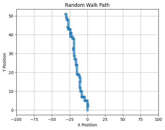
5 - Random Walk Simulation
Suppose your plane crushed, and want to predict where you will be after 100 steps. According to the wind, you know the probability of going forward, left or right.
class RandomWalkProblem:
def __init__(self, step_limit=100):
self.x_pos = 0
self.y_pos = 0
self.step_limit = step_limit
self.history = [(self.x_pos, self.y_pos)]
def run(self):
for _ in range(self.step_limit):
ransom_num = random.randint(0, 9)
if ransom_num <= 5:
self.y_pos += 1 # Move up
elif ransom_num <= 8:
self.x_pos -= 1 # Move left
else:
self.x_pos += 1 # Move right
self.history.append((self.x_pos, self.y_pos))
return (self.x_pos, self.y_pos)
def plot(self):
x_vals = [pos[0] for pos in self.history]
y_vals = [pos[1] for pos in self.history]
plt.plot(x_vals, y_vals, marker='o', alpha=0.5)
plt.title('Random Walk Path')
plt.xlabel('X Position')
plt.ylabel('Y Position')
plt.xlim(-self.step_limit, self.step_limit)
plt.grid()
plt.show()
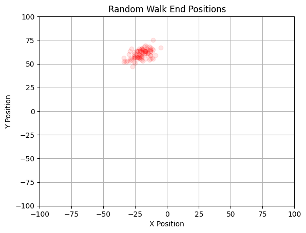
def multi_run(self, runs=10):
results = []
for _ in range(runs):
result = self.run()
results.append(result)
self.x_pos = 0
self.y_pos = 0
self.history = [(self.x_pos, self.y_pos)]
# print("Results of each run: ", results)
plt.plot([res[0] for res in results], [res[1] for res in results], 'ro', alpha=0.1)
plt.title('Random Walk End Positions')
plt.xlabel('X Position')
plt.ylabel('Y Position')
plt.xlim(-self.step_limit, self.step_limit)
plt.ylim(-self.step_limit, self.step_limit)
plt.grid()
plt.show()
if __name__ == "__main__":
walk = RandomWalkProblem(step_limit=100)
print("Final position after one run: ", walk.run())
walk.plot()
print("Final positions after multiple runs: ")
walk.multi_run(100)Final position after one run: (-31, 51)
Final positions after multiple runs:
What if you have z-axis as well?
class RandomWalk3D:
    def __init__(self, step_limit=100):
        self.x_pos = 0
        self.y_pos = 0
        self.z_pos = 0
        self.step_limit = step_limit
        self.history = [(self.x_pos, self.y_pos, self.z_pos)]

    def run(self):
        for _ in range(self.step_limit):
            random_num = random.randint(0, 5)
            if random_num == 0:
                self.x_pos += 1  # Move right
            elif random_num == 1:
                self.x_pos -= 1  # Move left
            elif random_num == 2:
                self.y_pos += 1  # Move forward
            elif random_num == 3:
                self.y_pos -= 1  # Move backward
            elif random_num == 4:
                self.z_pos += 1  # Move up
            else:
                self.z_pos -= 1  # Move down
            self.history.append((self.x_pos, self.y_pos, self.z_pos))
        return (self.x_pos, self.y_pos, self.z_pos)

    def plot(self):
        x_vals = [pos[0] for pos in self.history]
        y_vals = [pos[1] for pos in self.history]
        z_vals = [pos[2] for pos in self.history]

        fig = plt.figure()
        ax = fig.add_subplot(111, projection='3d')
        ax.plot(x_vals, y_vals, z_vals, marker='o')
        ax.set_title('3D Random Walk Path')
        ax.set_xlabel('X Position')
        ax.set_ylabel('Y Position')
        ax.set_zlabel('Z Position')
        plt.show()

    def multi_run(self, runs=10):
        results = []
        for _ in range(runs):
            result = self.run()
            results.append(result)
            self.x_pos = 0
            self.y_pos = 0
            self.z_pos = 0
            self.history = [(self.x_pos, self.y_pos, self.z_pos)]

        fig = plt.figure()
        ax = fig.add_subplot(111, projection='3d')
        ax.scatter([res[0] for res in results], [res[1] for res in results], [res[2] for res in results], c='r', alpha=0.5)
        ax.set_title('3D Random Walk End Positions')
        ax.set_xlabel('X Position')
        ax.set_ylabel('Y Position')
        ax.set_zlabel('Z Position')
        ax.set_xlim(-self.step_limit, self.step_limit)
        ax.set_ylim(-self.step_limit, self.step_limit)
        ax.set_zlim(-self.step_limit, self.step_limit)
        plt.show()

if __name__ == "__main__":
    walk_3d = RandomWalk3D(step_limit=100)
    walk_3d.multi_run(100)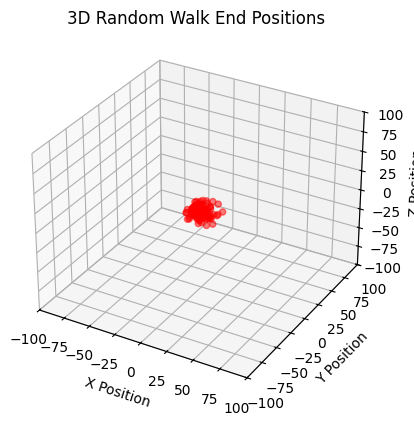
6 - Reliability Problem
A manufacturing plant has three bearings that fail according to a probability distribution. When a bearing fails, there is a delay before repair can begin. The plant must decide between two repair strategies:
Single Repair: Repair only the bearing(s) that have failed
All Repair: Replace all three bearings whenever any bearing fails
Each strategy has different costs associated with bearing replacement, downtime, and repairman labor. The goal is to simulate both strategies over a 30,000-hour period and determine which strategy minimizes total cost.
class ReliabilityProblem:
    def __init__(self, simulations=1000):
        self.simulations = simulations
        self.bearing_life_probabilities = {
            1000: 0.10,
            1100: 0.14,
            1200: 0.24,
            1300: 0.14,
            1400: 0.12,
            1500: 0.10,
            1600: 0.06,
            1700: 0.05,
            1800: 0.03,
            1900: 0.02,
        }

        self.delay_times_probabilities = {
            4: 0.30,
            6: 0.60,
            8: 0.10,
        }

    def run_single_repair(self, time_limit=30000):
        clock_1 = 0
        clock_2 = 0
        clock_3 = 0
        total_cost = 0

        for _ in range(self.simulations):
            life_1 = self.sample_from_distribution(self.bearing_life_probabilities)
            delay_1 = self.sample_from_distribution(self.delay_times_probabilities)
            clock_1 += life_1

            life_2 = self.sample_from_distribution(self.bearing_life_probabilities)
            delay_2 = self.sample_from_distribution(self.delay_times_probabilities)
            clock_2 += life_2

            life_3 = self.sample_from_distribution(self.bearing_life_probabilities)
            delay_3 = self.sample_from_distribution(self.delay_times_probabilities)
            clock_3 += life_3


            cost_of_bearings = 3 * 20

            total_delay = delay_1 + delay_2 + delay_3
            repair_delay = 0
            if clock_1 == clock_2 == clock_3:
                repair_delay += 40
            elif clock_1 == clock_2 or clock_2 == clock_3 or clock_1 == clock_3:
                repair_delay += 30 + 20
            else:
                repair_delay += 20 + 20 + 20
            downtime_cost = (total_delay + repair_delay) * 5

            # print("Clocks: ", clock_1, clock_2, clock_3, " Lives: ", life_1, life_2, life_3, " Delays: ", delay_1, delay_2, delay_3)
            repairman_cost = repair_delay * 25 / 60
            total_cost += cost_of_bearings + downtime_cost + repairman_cost

            if min(clock_1, clock_2, clock_3) >= time_limit:
                break

        return total_cost

    def run_all_repair(self, time_limit=30000):
        clock = 0
        total_delay = 0
        count = 0
        for _ in range(self.simulations):
            count += 1
            life_1 = self.sample_from_distribution(self.bearing_life_probabilities)
            life_2 = self.sample_from_distribution(self.bearing_life_probabilities)
            life_3 = self.sample_from_distribution(self.bearing_life_probabilities)
            clock += min(life_1, life_2, life_3)

            delay = self.sample_from_distribution(self.delay_times_probabilities)
            total_delay += delay
            # print("Clock: ", clock, " Lives: ", life_1, life_2, life_3, " delays: ", delay)

            if clock >= time_limit:
                break
        cost_of_bearings = 3 * count * 20
        downtime_cost = (total_delay + (count * 40)) * 5
        repairman_cost = (count * 40) * 25 / 60
        total_cost = cost_of_bearings + downtime_cost + repairman_cost
        return total_cost

    def sample_from_distribution(self, distribution):
        rand_value = random.random()
        cumulative_probability = 0.0
        for value, probability in distribution.items():
            cumulative_probability += probability
            if rand_value <= cumulative_probability:
                return value
        return value

if __name__ == "__main__":
    problem = ReliabilityProblem(simulations=300000)
    total_cost = problem.run_single_repair(30000)
    print("Total cost for single repair strategy over simulations: ", total_cost)
    total_cost_all_repair = problem.run_all_repair(30000)
    print("Total cost for all repair strategy over simulations: ", total_cost_all_repair)
Total cost for single repair strategy over simulations: 11676.666666666666
Total cost for all repair strategy over simulations: 8210.0
7 - Bombing Problem
hit_count = 0
miss_count = 0

mu = 0
sigma = 0.5

for _ in range(1_000_000):
    x_random = random.gauss(mu, sigma)
    y_random = random.gauss(mu, sigma)

    x_val = 500 * x_random
    y_val = 300 * y_random

    if (abs(x_val) <= 500) and (abs(y_val) <= 300):
        hit_count += 1
    else:
        miss_count += 1

strike_percentage = hit_count / (hit_count + miss_count) * 100
print("Strike Percentage:", strike_percentage)
Strike Percentage: 91.0601