Let’s think about simulating continuous systems. A continuous system is one that changes continuously over time, as opposed to discrete systems which change at specific intervals.
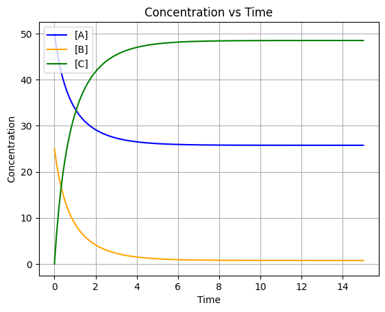
Chemical Reaction Simulation
This simulation models a reversible chemical reaction where compounds A and B react to form C. The system is governed by the following differential equations:
Then let’s try the Forward Euler Method, which is a first-order numerical procedure for solving ODEs. It approximates the derivative by using a small time step ():
Where:
is the forward reaction rate constant
is the reverse reaction rate constant
, , and represent the concentrations of compounds A, B, and C respectively
The simulation uses Euler’s method with a time step of to numerically integrate these equations over 15 time units, starting with initial concentrations , , and .
import matplotlib.pyplot as plt

class ChemicalReaction:
    def __init__(self, k1, k2, c1, c2, c3, time_diff=0.1):
        self.k1 = k1  # Rate constant for forward reaction
        self.k2 = k2  # Rate constant for reverse reaction
        self.c1 = c1  # Initial concentration of A
        self.c2 = c2  # Initial concentration of B
        self.c3 = c3  # Initial concentration of C
        self.time_diff = time_diff  # Time step for simulation

        self.time_points = [0]
        self.concentration_A = [c1]
        self.concentration_B = [c2]
        self.concentration_C = [c3]

    def simulate_reaction(self, total_time):
        steps = int(total_time / self.time_diff)
        for step in range(1, steps + 1):
            current_time = step * self.time_diff
            a = self.concentration_A[-1]
            b = self.concentration_B[-1]
            c = self.concentration_C[-1]

            # Calculate changes
            delta_a = (-self.k1 * a * b + self.k2 * c) * self.time_diff
            delta_b = (-self.k1 * a * b + self.k2 * c) * self.time_diff
            delta_c = 2 * (self.k1 * a * b - self.k2 * c) * self.time_diff

            # Update
            new_a = a + delta_a
            new_b = b + delta_b
            new_c = c + delta_c

            # Append
            self.time_points.append(current_time)
            self.concentration_A.append(new_a)
            self.concentration_B.append(new_b)
            self.concentration_C.append(new_c)

    def print_results(self):
        print("Time\t[A]\t[B]\t[C]")
        for t, a, b, c in zip(self.time_points, self.concentration_A, self.concentration_B, self.concentration_C):
            print(f"{t:.2f}\t{a:.4f}\t{b:.4f}\t{c:.4f}")

    def plot_concentrations(self):
        plt.plot(self.time_points, self.concentration_A, label='[A]', color='blue')
        plt.plot(self.time_points, self.concentration_B, label='[B]', color='orange')
        plt.plot(self.time_points, self.concentration_C, label='[C]', color='green')
        plt.title('Concentration vs Time')
        plt.xlabel('Time')
        plt.ylabel('Concentration')
        plt.legend()
        plt.grid()
        plt.show()

if __name__ == "__main__":
    reaction = ChemicalReaction(k1=0.025, k2=0.01, c1=50.0, c2=25.0, c3=0.0)
    reaction.simulate_reaction(total_time=15)
    reaction.print_results()
    reaction.plot_concentrations()
Time [A] [B] [C]
0.00 50.0000 25.0000 0.0000
0.10 46.8750 21.8750 6.2500
0.20 44.3178 19.3178 11.3645
0.30 42.1888 17.1888 15.6223
0.40 40.3915 15.3915 19.2170
0.50 38.8565 13.8565 22.2870
0.60 37.5328 12.5328 24.9345
0.70 36.3817 11.3817 27.2366
0.80 35.3737 10.3737 29.2525
0.90 34.4856 9.4856 31.0288
1.00 33.6988 8.6988 32.6023
1.10 32.9986 7.9986 34.0028
1.20 32.3727 7.3727 35.2545
1.30 31.8113 6.8113 36.3774
1.40 31.3060 6.3060 37.3880
1.50 30.8498 5.8498 38.3003
1.60 30.4370 5.4370 39.1261
1.70 30.0624 5.0624 39.8752
1.80 29.7218 4.7218 40.5564
1.90 29.4115 4.4115 41.1770
2.00 29.1283 4.1283 41.7434
2.10 28.8694 3.8694 42.2612
2.20 28.6324 3.6324 42.7352
2.30 28.4151 3.4151 43.1697
2.40 28.2157 3.2157 43.5686
2.50 28.0324 3.0324 43.9351
2.60 27.8639 2.8639 44.2723
2.70 27.7086 2.7086 44.5827
2.80 27.5656 2.5656 44.8688
2.90 27.4336 2.4336 45.1327
3.00 27.3119 2.3119 45.3763
3.10 27.1994 2.1994 45.6012
3.20 27.0954 2.0954 45.8091
3.30 26.9993 1.9993 46.0014
3.40 26.9104 1.9104 46.1793
3.50 26.8280 1.8280 46.3440
3.60 26.7518 1.7518 46.4965
3.70 26.6811 1.6811 46.6378
3.80 26.6156 1.6156 46.7688
3.90 26.5549 1.5549 46.8903
4.00 26.4985 1.4985 47.0029
4.10 26.4463 1.4463 47.1075
4.20 26.3978 1.3978 47.2045
4.30 26.3527 1.3527 47.2946
4.40 26.3109 1.3109 47.3782
4.50 26.2720 1.2720 47.4559
4.60 26.2359 1.2359 47.5281
4.70 26.2024 1.2024 47.5952
4.80 26.1712 1.1712 47.6575
4.90 26.1423 1.1423 47.7155
5.00 26.1153 1.1153 47.7693
5.10 26.0903 1.0903 47.8194
5.20 26.0670 1.0670 47.8660
5.30 26.0453 1.0453 47.9094
5.40 26.0252 1.0252 47.9497
5.50 26.0064 1.0064 47.9872
5.60 25.9890 0.9890 48.0221
5.70 25.9727 0.9727 48.0545
5.80 25.9576 0.9576 48.0847
5.90 25.9436 0.9436 48.1129
6.00 25.9305 0.9305 48.1390
6.10 25.9183 0.9183 48.1634
6.20 25.9070 0.9070 48.1861
6.30 25.8964 0.8964 48.2072
6.40 25.8866 0.8866 48.2268
6.50 25.8774 0.8774 48.2451
6.60 25.8689 0.8689 48.2622
6.70 25.8610 0.8610 48.2780
6.80 25.8536 0.8536 48.2928
6.90 25.8467 0.8467 48.3066
7.00 25.8403 0.8403 48.3194
7.10 25.8343 0.8343 48.3313
7.20 25.8288 0.8288 48.3424
7.30 25.8236 0.8236 48.3528
7.40 25.8188 0.8188 48.3624
7.50 25.8143 0.8143 48.3714
7.60 25.8101 0.8101 48.3797
7.70 25.8062 0.8062 48.3875
7.80 25.8026 0.8026 48.3948
7.90 25.7992 0.7992 48.4015
8.00 25.7961 0.7961 48.4078
8.10 25.7931 0.7931 48.4137
8.20 25.7904 0.7904 48.4192
8.30 25.7879 0.7879 48.4243
8.40 25.7855 0.7855 48.4290
8.50 25.7833 0.7833 48.4334
8.60 25.7812 0.7812 48.4375
8.70 25.7793 0.7793 48.4414
8.80 25.7775 0.7775 48.4449
8.90 25.7759 0.7759 48.4482
9.00 25.7743 0.7743 48.4513
9.10 25.7729 0.7729 48.4542
9.20 25.7715 0.7715 48.4569
9.30 25.7703 0.7703 48.4594
9.40 25.7691 0.7691 48.4618
9.50 25.7680 0.7680 48.4639
9.60 25.7670 0.7670 48.4660
9.70 25.7661 0.7661 48.4678
9.80 25.7652 0.7652 48.4696
9.90 25.7644 0.7644 48.4712
10.00 25.7636 0.7636 48.4728
10.10 25.7629 0.7629 48.4742
10.20 25.7622 0.7622 48.4755
10.30 25.7616 0.7616 48.4767
10.40 25.7611 0.7611 48.4779
10.50 25.7605 0.7605 48.4790
10.60 25.7600 0.7600 48.4800
10.70 25.7596 0.7596 48.4809
10.80 25.7591 0.7591 48.4818
10.90 25.7587 0.7587 48.4826
11.00 25.7583 0.7583 48.4833
11.10 25.7580 0.7580 48.4840
11.20 25.7577 0.7577 48.4847
11.30 25.7574 0.7574 48.4853
11.40 25.7571 0.7571 48.4859
11.50 25.7568 0.7568 48.4864
11.60 25.7566 0.7566 48.4869
11.70 25.7563 0.7563 48.4873
11.80 25.7561 0.7561 48.4878
11.90 25.7559 0.7559 48.4882
12.00 25.7557 0.7557 48.4885
12.10 25.7556 0.7556 48.4889
12.20 25.7554 0.7554 48.4892
12.30 25.7553 0.7553 48.4895
12.40 25.7551 0.7551 48.4898
12.50 25.7550 0.7550 48.4900
12.60 25.7549 0.7549 48.4903
12.70 25.7547 0.7547 48.4905
12.80 25.7546 0.7546 48.4907
12.90 25.7545 0.7545 48.4909
13.00 25.7545 0.7545 48.4911
13.10 25.7544 0.7544 48.4913
13.20 25.7543 0.7543 48.4914
13.30 25.7542 0.7542 48.4916
13.40 25.7541 0.7541 48.4917
13.50 25.7541 0.7541 48.4918
13.60 25.7540 0.7540 48.4920
13.70 25.7540 0.7540 48.4921
13.80 25.7539 0.7539 48.4922
13.90 25.7539 0.7539 48.4923
14.00 25.7538 0.7538 48.4924
14.10 25.7538 0.7538 48.4924
14.20 25.7537 0.7537 48.4925
14.30 25.7537 0.7537 48.4926
14.40 25.7537 0.7537 48.4927
14.50 25.7536 0.7536 48.4927
14.60 25.7536 0.7536 48.4928
14.70 25.7536 0.7536 48.4928
14.80 25.7536 0.7536 48.4929
14.90 25.7535 0.7535 48.4929
15.00 25.7535 0.7535 48.4930
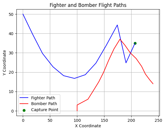
Pure Pursuit Simulation
2D Version
1. The Geometry of Pursuit
At any given time step , the fighter is at coordinates and the bomber is at . The line of sight (LOS) is the vector connecting these two points.
The distance between them is calculated using the Pythagorean theorem:
2. Heading Angle ()
To intercept the target, the fighter must align its velocity vector with the current line of sight. The angle of this vector relative to the x-axis is determined by the trigonometry of the triangle formed by the two positions:
Sine:
Cosine:
3. Iterative Kinematic Update
Because the system is discrete (simulated step-by-step), we update the fighter’s position using its constant speed . For a small time step (implicitly handled by your iteration loop), the new position is calculated by projecting the velocity vector:
import math
import matplotlib.pyplot as plt

# Fighter coordinates
xf = [0]
yf = [50]
speed = 20  # Fighter speed
capture_distance = 10  # Distance at which the fighter captures the bomber

# Bomber coordinates
xb = [100, 100, 120, 129, 140, 149, 158, 168, 179, 188, 198, 209, 219, 226, 234, 240]
yb = [0, 3, 6, 10, 15, 20, 26, 32, 37, 34, 30, 27, 23, 19, 16, 14]

def calc_distance(x1, y1, x2, y2):
    return math.sqrt((x2 - x1) ** 2 + (y2 - y1) ** 2)

def sin_theta(x1, y1, x2, y2):
    return (y2 - y1) / calc_distance(x1, y1, x2, y2)

def cos_theta(x1, y1, x2, y2):
    return (x2 - x1) / calc_distance(x1, y1, x2, y2)

def simulate_flight():
    global xf, yf, xb, yb, speed, capture_distance
    iteration = 0

    while True:
        xf = xf + [xf[-1] + speed * cos_theta(xf[-1], yf[-1], xb[iteration], yb[iteration])]
        yf = yf + [yf[-1] + speed * sin_theta(xf[-1], yf[-1], xb[iteration], yb[iteration])]

        distance = calc_distance(xf[iteration], yf[iteration], xb[iteration], yb[iteration])
        print("Iteration:", iteration+1, "Distance:", distance)
        iteration += 1
        if distance <= capture_distance or len(xf) >= len(xb):
            break

def plot_flight():
    plt.plot(xf, yf, label='Fighter Path', color='blue')
    plt.plot(xb, yb, label='Bomber Path', color='red')
    plt.scatter(xf[-1], yf[-1], color='green', label='Capture Point')
    plt.title('Fighter and Bomber Flight Paths')
    plt.xlabel('X Coordinate')
    plt.ylabel('Y Coordinate')
    plt.legend()
    plt.grid()
    plt.show()

def plot_fight_animation():
    plt.ion()
    fig, ax = plt.subplots()
    ax.set_xlim(0, 250)
    ax.set_ylim(0, 100)
    fighter_line, = ax.plot([], [], 'b-', label='Fighter Path')
    bomber_line, = ax.plot([], [], 'r-', label='Bomber Path')
    fighter_point, = ax.plot([], [], 'bo', label='Fighter')
    bomber_point, = ax.plot([], [], 'ro', label='Bomber')
    ax.legend()
    ax.grid()

    for i in range(len(xf)):
        fighter_line.set_data(xf[:i+1], yf[:i+1])
        bomber_line.set_data(xb[:i+1], yb[:i+1])
        fighter_point.set_data(xf[:i], yf[:i])
        bomber_point.set_data(xb[:i], yb[:i])
        plt.pause(0.5)

    plt.ioff()
    plt.show()

simulate_flight()
plot_flight()

# Run the animation in a single file for better compatibility
# plot_fight_animation()
Iteration: 1 Distance: 111.80339887498948
Iteration: 2 Distance: 89.89836784312963
Iteration: 3 Distance: 87.11594981353471
Iteration: 4 Distance: 74.69560058571354
Iteration: 5 Distance: 64.96670435422362
Iteration: 6 Distance: 54.010853327288075
Iteration: 7 Distance: 43.57236123303999
Iteration: 8 Distance: 34.03104671890206
Iteration: 9 Distance: 24.872229621894245
Iteration: 10 Distance: 17.296424694649446
Iteration: 11 Distance: 9.407161735497592
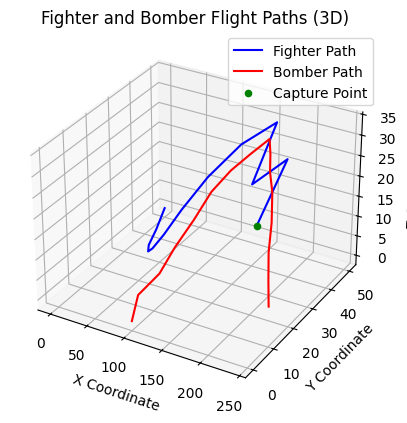
3D Version
The distance between the fighter and the bomber is now the magnitude of the displacement vector in 3D space:
import math
from mpl_toolkits.mplot3d import Axes3D

import matplotlib.pyplot as plt

# Fighter coordinates
xf = [0]
yf = [50]
zf = [0]
speed = 20  # Fighter speed
capture_distance = 10  # Distance at which the fighter captures the bomber

# Bomber coordinates
xb = [100, 100, 120, 129, 140, 149, 158, 168, 179, 188, 198, 209, 219, 226, 234, 240]
yb = [0, 3, 6, 10, 15, 20, 26, 32, 37, 34, 30, 27, 23, 19, 16, 14]
zb = [0, 5, 10, 15, 20, 25, 28, 30, 32, 30, 28, 25, 20, 15, 10, 5]

def calc_distance(x1, y1, z1, x2, y2, z2):
    return math.sqrt((x2 - x1) ** 2 + (y2 - y1) ** 2 + (z2 - z1) ** 2)

def sin_theta(x1, y1, z1, x2, y2, z2):
    return (y2 - y1) / calc_distance(x1, y1, z1, x2, y2, z2)

def cos_theta(x1, y1, z1, x2, y2, z2):
    return (x2 - x1) / calc_distance(x1, y1, z1, x2, y2, z2)

def sin_phi(x1, y1, z1, x2, y2, z2):
    return (z2 - z1) / calc_distance(x1, y1, z1, x2, y2, z2)

def simulate_flight():
    global xf, yf, zf, xb, yb, zb, speed, capture_distance
    iteration = 0

    while True:
        xf = xf + [xf[-1] + speed * cos_theta(xf[-1], yf[-1], zf[-1], xb[iteration], yb[iteration], zb[iteration])]
        yf = yf + [yf[-1] + speed * sin_theta(xf[-1], yf[-1], zf[-1], xb[iteration], yb[iteration], zb[iteration])]
        zf = zf + [zf[-1] + speed * sin_phi(xf[-1], yf[-1], zf[-1], xb[iteration], yb[iteration], zb[iteration])]

        distance = calc_distance(xf[iteration], yf[iteration], zf[iteration], xb[iteration], yb[iteration], zb[iteration])
        print("Iteration:", iteration+1, "Distance:", distance)
        iteration += 1
        if distance <= capture_distance or len(xf) >= len(xb):
            break

def plot_flight():
    fig = plt.figure()
    ax = fig.add_subplot(111, projection='3d')
    ax.plot(xf, yf, zf, label='Fighter Path', color='blue')
    ax.plot(xb, yb, zb, label='Bomber Path', color='red')
    ax.scatter(xf[-1], yf[-1], zf[-1], color='green', label='Capture Point')
    ax.set_title('Fighter and Bomber Flight Paths (3D)')
    ax.set_xlabel('X Coordinate')
    ax.set_ylabel('Y Coordinate')
    ax.set_zlabel('Z Coordinate')
    ax.legend()
    plt.show()

def plot_fight_animation():
    plt.ion()
    fig = plt.figure()
    ax = fig.add_subplot(111, projection='3d')
    ax.set_xlim(0, 250)
    ax.set_ylim(0, 100)
    ax.set_zlim(0, 40)
    fighter_line, = ax.plot([], [], [], 'b-', label='Fighter Path')
    bomber_line, = ax.plot([], [], [], 'r-', label='Bomber Path')
    fighter_point, = ax.plot([], [], [], 'bo', label='Fighter')
    bomber_point, = ax.plot([], [], [], 'ro', label='Bomber')
    ax.set_xlabel('X')
    ax.set_ylabel('Y')
    ax.set_zlabel('Z')
    ax.legend()
    ax.grid()

    for i in range(len(xf)):
        fighter_line.set_data(xf[:i+1], yf[:i+1])
        fighter_line.set_3d_properties(zf[:i+1])
        bomber_line.set_data(xb[:i+1], yb[:i+1])
        bomber_line.set_3d_properties(zb[:i+1])
        fighter_point.set_data([xf[i]], [yf[i]])
        fighter_point.set_3d_properties([zf[i]])
        bomber_point.set_data([xb[i]], [yb[i]])
        bomber_point.set_3d_properties([zb[i]])
        plt.pause(0.5)

    plt.ioff()
    plt.show()

simulate_flight()
plot_flight()
Iteration: 1 Distance: 111.80339887498948
Iteration: 2 Distance: 90.0373063838465
Iteration: 3 Distance: 87.56947209689841
Iteration: 4 Distance: 75.63662428124731
Iteration: 5 Distance: 66.41726456828744
Iteration: 6 Distance: 55.96349153539731
Iteration: 7 Distance: 45.5004092954095
Iteration: 8 Distance: 35.82864253435405
Iteration: 9 Distance: 26.64790269913945
Iteration: 10 Distance: 18.407471214949947
Iteration: 11 Distance: 10.295713805036083
Iteration: 12 Distance: 9.945906440073788
Serial Chase Simulation
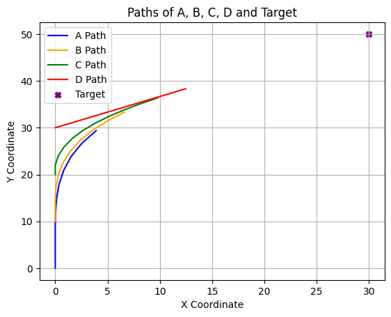
A group of moving objects are arranged in a serial pursuit chain where each object chases the one ahead of it: A chases B, B chases C, and C chases D. Each object moves directly toward its target, independent of the fact that it is being pursued by another object. The chase concludes the moment any hit (defined as a distance of less than 0.005 units between a pursuer and its target) occurs.
The initial conditions for the objects are:
Object A: Located at with a constant velocity of .
Object B: Located at with a constant velocity of .
Object C: Located at with a constant velocity of .
Object D: Located at with a constant velocity of .
The movement behavior is defined as follows:
Object D moves constantly toward a fixed target point located at .
Object C moves constantly in a direction pointing toward the instantaneous position of Object D.
Object B moves constantly in a direction pointing toward the instantaneous position of Object C.
Object A moves constantly in a direction pointing toward the instantaneous position of Object B.
Identify which object will hit its target first, and calculate the elapsed time at the moment the first hit occurs.
import math
import matplotlib.pyplot as plt

A, B, C, D = (0, 0), (0,10), (0,20), (0,30)

A_history = [A]
B_history = [B]
C_history = [C]
D_history = [D]

vA, vB, vC, vD = 30, 25, 20, 15
target_d = (30, 50)

def distance(p1, p2):
    return math.sqrt((p1[0] - p2[0])**2 + (p1[1] - p2[1])**2)

t = 0

for i in range(10):
    t += 0.1

    # Move A towards B
    a_to_b = distance(A, B)
    if a_to_b < 0.005:
        print(f"A hits B at time {t:.2f} hours")
        break
    A = (A[0] + vA * 0.1 * (B[0] - A[0]) / a_to_b, A[1] + vA * 0.1 * (B[1] - A[1]) / a_to_b)
    A_history.append(A)

    # Move B towards C
    b_to_c = distance(B, C)
    if b_to_c < 0.005:
        print(f"B hits C at time {t:.2f} hours")
        break
    B = (B[0] + vB * 0.1 * (C[0] - B[0]) / b_to_c, B[1] + vB * 0.1 * (C[1] - B[1]) / b_to_c)
    B_history.append(B)

    # Move C towards D
    c_to_d = distance(C, D)
    if c_to_d < 0.005:
        print(f"C hits D at time {t:.2f} hours")
        break
    C = (C[0] + vC * 0.1 * (D[0] - C[0]) / c_to_d, C[1] + vC * 0.1 * (D[1] - C[1]) / c_to_d)
    C_history.append(C)

    # Move D towards target
    d_to_target = distance(D, target_d)
    if d_to_target < 0.005:
        print(f"D hits the target at time {t:.2f} hours")
        break
    D = (D[0] + vD * 0.1 * (target_d[0] - D[0]) / d_to_target, D[1] + vD * 0.1 * (target_d[1] - D[1]) / d_to_target)
    D_history.append(D)

    # Preety-Print
    print(f"T: {t:.2f},\n A: ({A[0]:.2f}, {A[1]:.2f}), B: ({B[0]:.2f}, {B[1]:.2f}), C: ({C[0]:.2f}, {C[1]:.2f}), D: ({D[0]:.2f}, {D[1]:.2f}), AB: {a_to_b:.2f}, BC: {b_to_c:.2f}, CD: {c_to_d:.2f}, DTarget: {d_to_target:.2f}\n")

# Plotting the paths
plt.plot(*zip(*A_history), label='A Path', color='blue')
plt.plot(*zip(*B_history), label='B Path', color='orange')
plt.plot(*zip(*C_history), label='C Path', color='green')
plt.plot(*zip(*D_history), label='D Path', color='red')
plt.scatter(target_d[0], target_d[1], color='purple', label='Target', marker='X')
plt.title('Paths of A, B, C, D and Target')
plt.xlabel('X Coordinate')
plt.ylabel('Y Coordinate')
plt.legend()
plt.grid()
plt.show()
T: 0.10,
A: (0.00, 3.00), B: (0.00, 12.50), C: (0.00, 22.00), D: (1.25, 30.83), AB: 10.00, BC: 10.00, CD: 10.00, DTarget: 36.06
T: 0.20,
A: (0.00, 6.00), B: (0.00, 15.00), C: (0.28, 23.98), D: (2.50, 31.66), AB: 9.50, BC: 9.50, CD: 8.92, DTarget: 34.56
T: 0.30,
A: (0.00, 9.00), B: (0.08, 17.50), C: (0.83, 25.90), D: (3.74, 32.50), AB: 9.00, BC: 8.98, CD: 8.00, DTarget: 33.06
T: 0.40,
A: (0.03, 12.00), B: (0.30, 19.99), C: (1.64, 27.73), D: (4.99, 33.33), AB: 8.50, BC: 8.44, CD: 7.21, DTarget: 31.56
T: 0.50,
A: (0.13, 15.00), B: (0.73, 22.45), C: (2.67, 29.45), D: (6.24, 34.16), AB: 7.99, BC: 7.86, CD: 6.52, DTarget: 30.06
T: 0.60,
A: (0.37, 17.99), B: (1.40, 24.86), C: (3.88, 31.04), D: (7.49, 34.99), AB: 7.48, BC: 7.26, CD: 5.91, DTarget: 28.56
T: 0.70,
A: (0.81, 20.96), B: (2.33, 27.18), C: (5.23, 32.52), D: (8.74, 35.82), AB: 6.95, BC: 6.66, CD: 5.35, DTarget: 27.06
T: 0.80,
A: (1.52, 23.87), B: (3.52, 29.38), C: (6.68, 33.89), D: (9.98, 36.66), AB: 6.41, BC: 6.07, CD: 4.82, DTarget: 25.56
T: 0.90,
A: (2.55, 26.69), B: (4.96, 31.43), C: (8.22, 35.17), D: (11.23, 37.49), AB: 5.86, BC: 5.51, CD: 4.31, DTarget: 24.06
T: 1.00,
A: (3.91, 29.36), B: (6.60, 33.31), C: (9.80, 36.39), D: (12.48, 38.32), AB: 5.31, BC: 4.97, CD: 3.80, DTarget: 22.56