Basic Image Enhancement Using Mathematical Operations

Image Processing techniques take advantage of mathematical operations to achieve different results. Most often we arrive at an enhanced version of the image using some basic operations. We will take a look at some of the fundamental operations often used in computer vision pipelines. In this notebook we will cover:

Arithmetic Operations like addition, multiplication
Thresholding & Masking
Bitwise Operations like OR, AND, XOR

import os
import cv2
import numpy as np
import matplotlib.pyplot as plt

from zipfile import ZipFile
from urllib.request import urlretrieve

from IPython.display import Image

%matplotlib inline

Download Assets¶

def download_and_unzip(url, save_path):
    print(f"Downloading and extracting assests....", end="")

    # Downloading zip file using urllib package.
    urlretrieve(url, save_path)

    try:
        # Extracting zip file using the zipfile package.
        with ZipFile(save_path) as z:
            # Extract ZIP file contents in the same directory.
            z.extractall(os.path.split(save_path)[0])

        print("Done")

    except Exception as e:
        print("\nInvalid file.", e)

URL = r"https://www.dropbox.com/s/0oe92zziik5mwhf/opencv_bootcamp_assets_NB4.zip?dl=1"

asset_zip_path = os.path.join(os.getcwd(), "opencv_bootcamp_assets_NB4.zip")

# Download if assest ZIP does not exists.
if not os.path.exists(asset_zip_path):
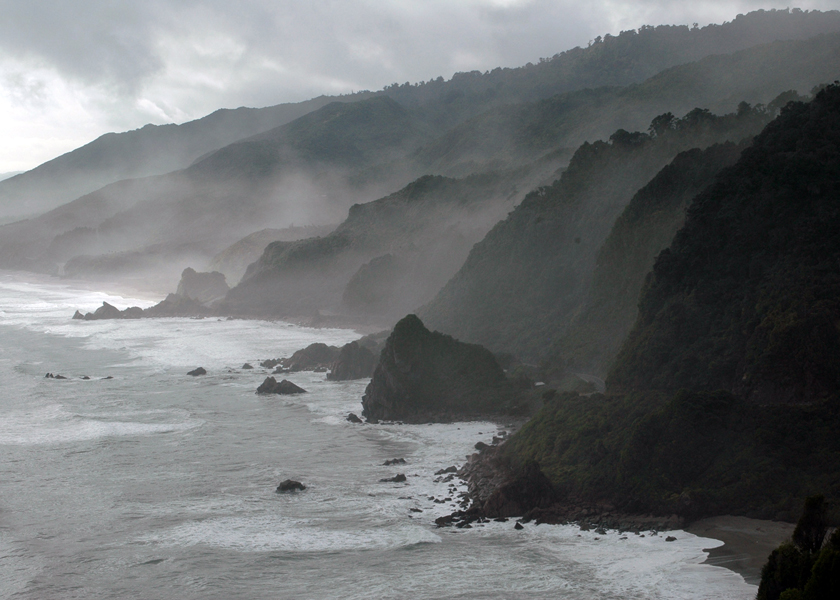
    download_and_unzip(URL, asset_zip_path)

Original image¶

img_bgr = cv2.imread("New_Zealand_Coast.jpg", cv2.IMREAD_COLOR)
img_rgb = cv2.cvtColor(img_bgr, cv2.COLOR_BGR2RGB)
print(img_rgb.shape)

# Display 18x18 pixel image.
Image(filename="New_Zealand_Coast.jpg")

(600, 840, 3)

Addition or Brightness¶

The first operation we discuss is simple addition of images. This results in increasing or decreasing the brightness of the image since we are eventually increasing or decreasing the intensity values of each pixel by the same amount. So, this will result in a global increase/decrease in brightness.

matrix = np.ones(img_rgb.shape, dtype="uint8") * 50

img_rgb_brighter = cv2.add(img_rgb, matrix)
img_rgb_darker   = cv2.subtract(img_rgb, matrix)


# Show the images
plt.figure(figsize=[18, 5])
plt.subplot(131); plt.imshow(img_rgb_darker);  plt.title("Darker");
plt.subplot(132); plt.imshow(img_rgb);         plt.title("Original");
plt.subplot(133); plt.imshow(img_rgb_brighter);plt.title("Brighter");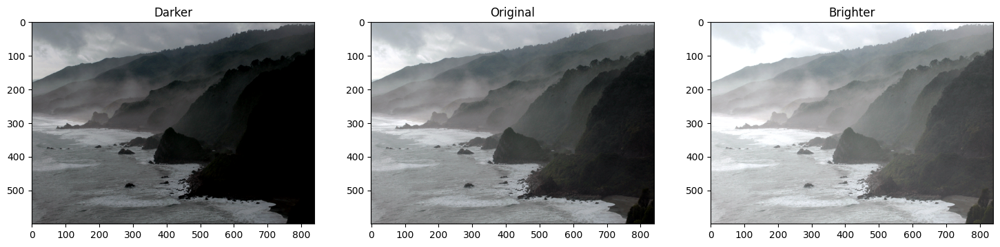

Multiplication or Contrast¶

Just like addition can result in brightness change, multiplication can be used to improve the contrast of the image.

Contrast is the difference in the intensity values of the pixels of an image. Multiplying the intensity values with a constant can make the difference larger or smaller ( if multiplying factor is < 1 ).

matrix_low_contrast = np.ones(img_rgb.shape) * 0.8
matrix_high_contast = np.ones(img_rgb.shape) * 1.2

img_rgb_darker   = np.uint8(cv2.multiply(np.float64(img_rgb), matrix_low_contrast))
img_rgb_brighter = np.uint8(cv2.multiply(np.float64(img_rgb), matrix_high_contast))

# Show the images
plt.figure(figsize=[18,5])
plt.subplot(131); plt.imshow(img_rgb_darker);  plt.title("Lower Contrast");
plt.subplot(132); plt.imshow(img_rgb);         plt.title("Original");
plt.subplot(133); plt.imshow(img_rgb_brighter);plt.title("Higher Contrast");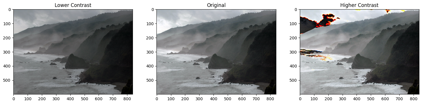

What happened?¶

Can you see the weird colors in some areas of the image after multiplication?

The issue is that after multiplying, the values which are already high, are becoming greater than 255. Thus, the overflow issue. How do we overcome this?

Handling Overflow using np.clip¶

matrix_low_contrast = np.ones(img_rgb.shape) * 0.8
matrix_high_contast = np.ones(img_rgb.shape) * 1.2

img_rgb_lower  = np.uint8(cv2.multiply(np.float64(img_rgb), matrix_low_contrast))
img_rgb_higher = np.uint8(np.clip(cv2.multiply(np.float64(img_rgb), matrix_high_contast), 0, 255))

# Show the images
plt.figure(figsize=[18,5])
plt.subplot(131); plt.imshow(img_rgb_lower); plt.title("Lower Contrast");
plt.subplot(132); plt.imshow(img_rgb);       plt.title("Original");
plt.subplot(133); plt.imshow(img_rgb_higher);plt.title("Higher Contrast");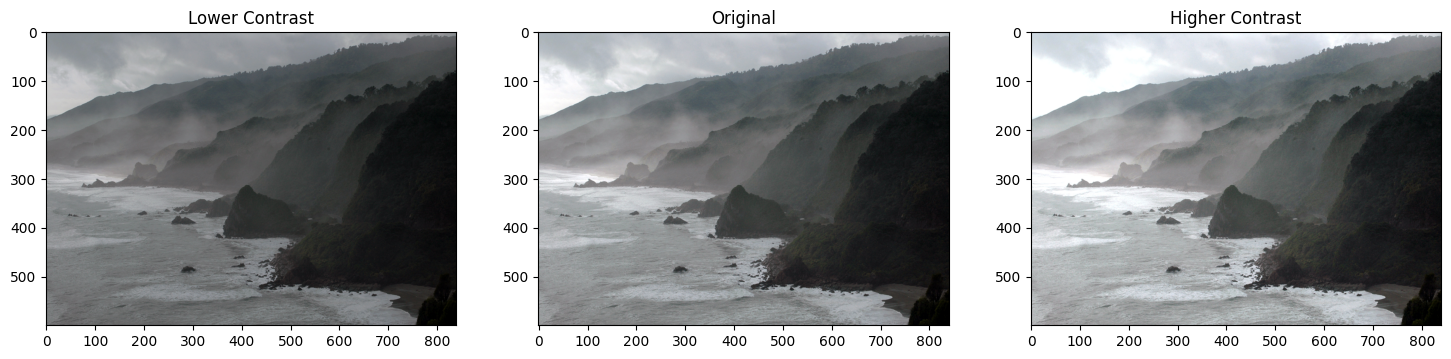

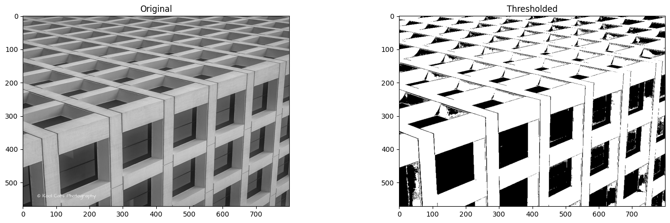
Image Thresholding¶

Binary Images have a lot of use cases in Image Processing. One of the most common use cases is that of creating masks. Image Masks allow us to process on specific parts of an image keeping the other parts intact. Image Thresholding is used to create Binary Images from grayscale images. You can use different thresholds to create different binary images from the same original image.

Function Syntax¶

retval, dst = cv2.threshold( src, thresh, maxval, type[, dst] )

dst: The output array of the same size and type and the same number of channels as src.

The function has 4 required arguments:

src: input array (multiple-channel, 8-bit or 32-bit floating point).
thresh: threshold value.
maxval: maximum value to use with the THRESH_BINARY and THRESH_BINARY_INV thresholding types.
type: thresholding type (see ThresholdTypes).

OpenCV Documentation¶

Documentation link

img_read = cv2.imread("building-windows.jpg", cv2.IMREAD_GRAYSCALE)
retval, img_thresh = cv2.threshold(img_read, 100, 255, cv2.THRESH_BINARY)
print(retval)

# Show the images
plt.figure(figsize=[18, 5])

plt.subplot(121);plt.imshow(img_read, cmap="gray");  plt.title("Original")
plt.subplot(122);plt.imshow(img_thresh, cmap="gray");plt.title("Thresholded")

print(img_thresh.shape)

100.0
(572, 800)

Application: Sheet Music Reader¶

Suppose you wanted to build an application that could read (decode) sheet music. This is similar to Optical Character Recognigition (OCR) for text documents where the goal is to recognize text characters. In either application, one of the first steps in the processing pipeline is to isolate the important information in the image of a document (separating it from the background). This task can be accomplished with thresholding techniques. Let’s take a look at an example.

Function Syntax¶

dst = cv.adaptiveThreshold( src, maxValue, adaptiveMethod, thresholdType, blockSize, C[, dst] )

dst Destination image of the same size and the same type as src.

The function has 6 required arguments:

src: Source 8-bit single-channel image.
maxValue: Non-zero value assigned to the pixels for which the condition is satisfied
adaptiveMethod: Adaptive thresholding algorithm to use, see AdaptiveThresholdTypes. The BORDER_REPLICATE | BORDER_ISOLATED is used to process boundaries.
thresholdType: Thresholding type that must be either THRESH_BINARY or THRESH_BINARY_INV, see ThresholdTypes.
blockSize: Size of a pixel neighborhood that is used to calculate a threshold value for the pixel: 3, 5, 7, and so on.
C: Constant subtracted from the mean or weighted mean (see the details below). Normally, it is positive but may be zero or negative as well.

# Read the original image
img_read = cv2.imread("Piano_Sheet_Music.png", cv2.IMREAD_GRAYSCALE)

# Perform global thresholding
retval, img_thresh_gbl_1 = cv2.threshold(img_read, 50, 255, cv2.THRESH_BINARY)

# Perform global thresholding
retval, img_thresh_gbl_2 = cv2.threshold(img_read, 130, 255, cv2.THRESH_BINARY)

# Perform adaptive thresholding
img_thresh_adp = cv2.adaptiveThreshold(img_read, 255, cv2.ADAPTIVE_THRESH_MEAN_C, cv2.THRESH_BINARY, 11, 7)

# Show the images
plt.figure(figsize=[18,15])
plt.subplot(221); plt.imshow(img_read,        cmap="gray");  plt.title("Original");
plt.subplot(222); plt.imshow(img_thresh_gbl_1,cmap="gray");  plt.title("Thresholded (global: 50)");
plt.subplot(223); plt.imshow(img_thresh_gbl_2,cmap="gray");  plt.title("Thresholded (global: 130)");
plt.subplot(224); plt.imshow(img_thresh_adp,  cmap="gray");  plt.title("Thresholded (adaptive)");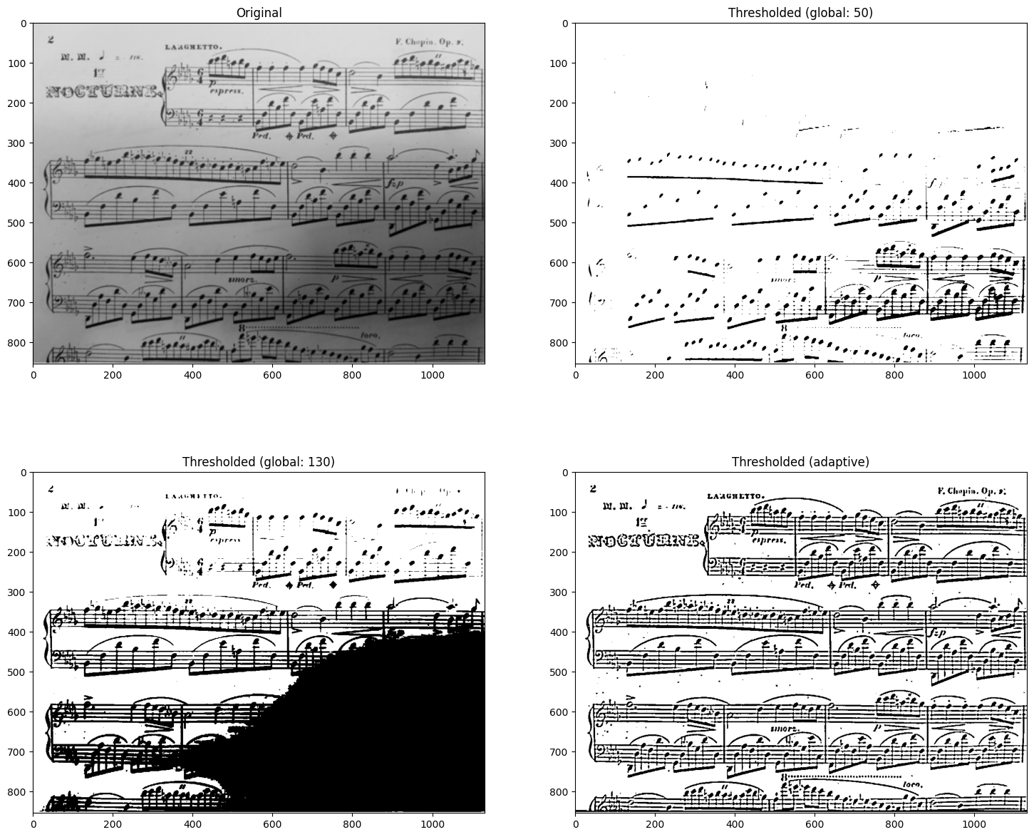

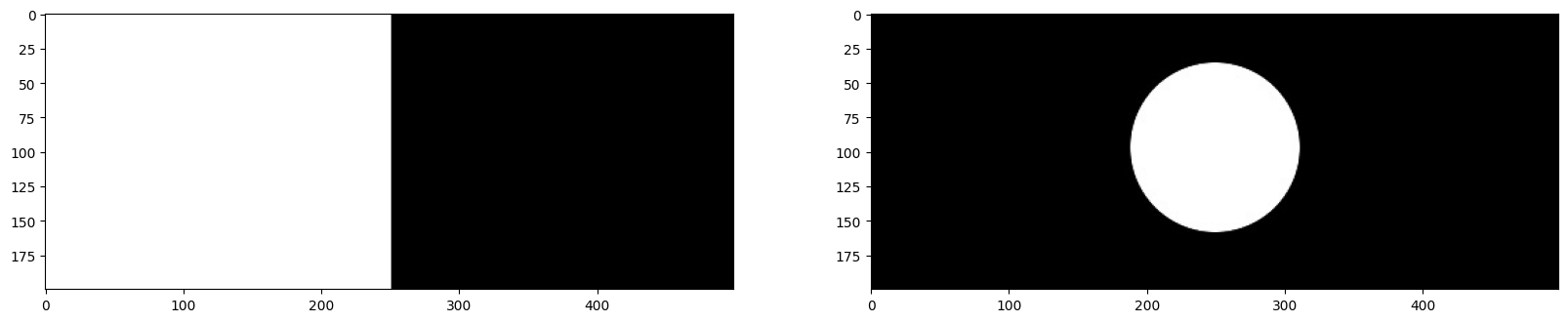
Bitwise Operations¶

Function Syntax¶

Example API for cv2.bitwise_and(). Others include: cv2.bitwise_or(), cv2.bitwise_xor(), cv2.bitwise_not()

dst = cv2.bitwise_and( src1, src2[, dst[, mask]] )

dst: Output array that has the same size and type as the input arrays.

The function has 2 required arguments:

src1: first input array or a scalar.
src2: second input array or a scalar.

An important optional argument is:

mask: optional operation mask, 8-bit single channel array, that specifies elements of the output array to be changed.

OpenCV Documentation¶

img_rec = cv2.imread("rectangle.jpg", cv2.IMREAD_GRAYSCALE)

img_cir = cv2.imread("circle.jpg", cv2.IMREAD_GRAYSCALE)

plt.figure(figsize=[20, 5])
plt.subplot(121);plt.imshow(img_rec, cmap="gray")
plt.subplot(122);plt.imshow(img_cir, cmap="gray")
print(img_rec.shape)

(200, 499)

Bitwise AND Operator¶

result = cv2.bitwise_and(img_rec, img_cir, mask=None)
plt.imshow(result, cmap="gray")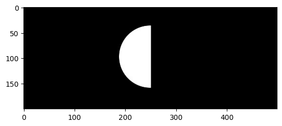

Bitwise OR Operator¶

result = cv2.bitwise_or(img_rec, img_cir, mask=None)
plt.imshow(result, cmap="gray")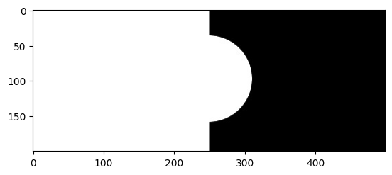

Bitwise XOR Operator¶

result = cv2.bitwise_xor(img_rec, img_cir, mask=None)
plt.imshow(result, cmap="gray")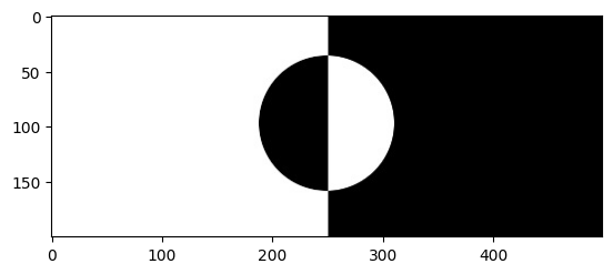

Application: Logo Manipulation¶

In this section we will show you how to fill in the white lettering of the Coca-Cola logo below with a background image.

Image(filename='Logo_Manipulation.png')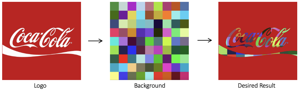

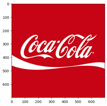
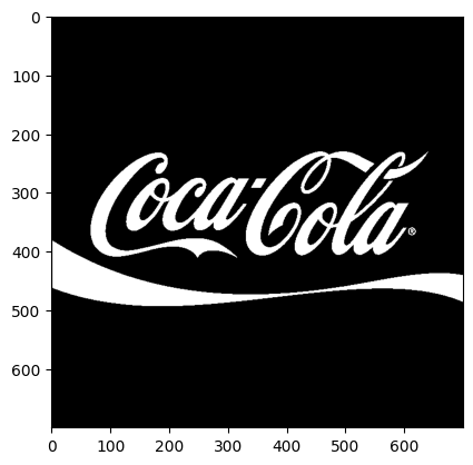
Read Foreground image¶

img_bgr = cv2.imread("coca-cola-logo.png")
img_rgb = cv2.cvtColor(img_bgr, cv2.COLOR_BGR2RGB)
plt.imshow(img_rgb)

print(img_rgb.shape)

logo_h = img_rgb.shape[0]
logo_w = img_rgb.shape[1]

(700, 700, 3)

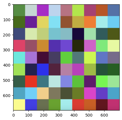
Read Background image¶

# Read in image of color cheackerboad background
img_background_bgr = cv2.imread("checkerboard_color.png")
img_background_rgb = cv2.cvtColor(img_background_bgr, cv2.COLOR_BGR2RGB)

# Resize background image to same size as logo image
img_background_rgb = cv2.resize(img_background_rgb, (logo_w, logo_h), interpolation=cv2.INTER_AREA)

plt.imshow(img_background_rgb)
print(img_background_rgb.shape)

(700, 700, 3)

Create Mask for original Image¶

img_gray = cv2.cvtColor(img_rgb, cv2.COLOR_RGB2GRAY)

# Apply global thresholding to create a binary mask of the logo
retval, img_mask = cv2.threshold(img_gray, 127, 255, cv2.THRESH_BINARY)

plt.imshow(img_mask, cmap="gray")
print(img_mask.shape)

(700, 700)

Invert the Mask¶

# Create an inverse mask
img_mask_inv = cv2.bitwise_not(img_mask)
plt.imshow(img_mask_inv, cmap="gray")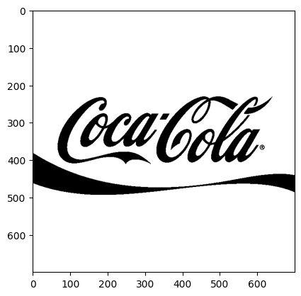

Apply background on the Mask¶

# Create colorful background "behind" the logo lettering
img_background = cv2.bitwise_and(img_background_rgb, img_background_rgb, mask=img_mask)
plt.imshow(img_background)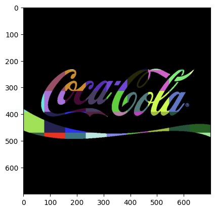

Isolate foreground from image¶

# Isolate foreground (red from original image) using the inverse mask
img_foreground = cv2.bitwise_and(img_rgb, img_rgb, mask=img_mask_inv)
plt.imshow(img_foreground)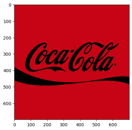

Result: Merge Foreground and Background¶

# Add the two previous results obtain the final result
result = cv2.add(img_background, img_foreground)
plt.imshow(result)
cv2.imwrite("logo_final.png", result[:, :, ::-1])

True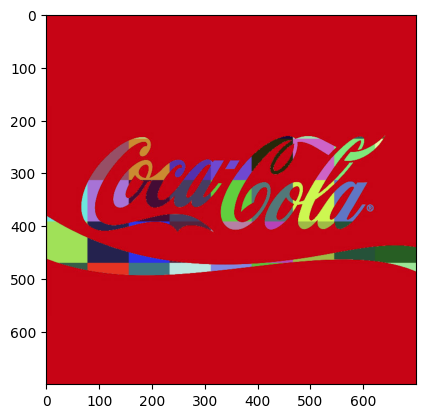

arr1 = np.array([200, 250], dtype=np.uint8).reshape(-1, 1)
arr2 = np.array([40, 40], dtype=np.uint8).reshape(-1, 1)
print(arr1)
print(arr2)

add_numpy = arr1+arr2
add_cv2 = cv2.add(arr1, arr2)

[[200]
 [250]]
[[40]
 [40]]

print(add_numpy)
print(add_cv2)

[[240]
 [ 34]]
[[240]
 [255]]