import pandas as pd
import matplotlib.pyplot as plt
import seaborn as sns
load_dataset()
Seaborn comes with a handy way to quickly get some datasets to play with, but please note this is NOT the normal way of loading a CSV file. Usually we’d use pandas.read_csv() as we’ve seen so far.
tips = sns.load_dataset("tips")tipsLoading...
penguins = sns.load_dataset("penguins")Seaborn Scatterplots
sns.set_theme()sns.scatterplot(data=tips, x="total_bill", y="tip")<Axes: xlabel='total_bill', ylabel='tip'>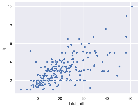
tips.plot(kind="scatter", x="total_bill", y="tip")<Axes: xlabel='total_bill', ylabel='tip'>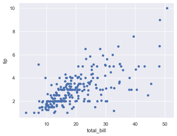
sns.scatterplot(data=tips, x="total_bill", y="tip", hue="smoker")<Axes: xlabel='total_bill', ylabel='tip'>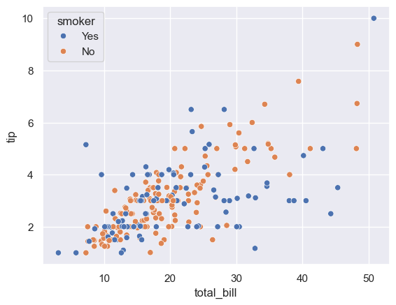
sns.scatterplot(data=tips, x="total_bill", y="tip", hue="sex")<Axes: xlabel='total_bill', ylabel='tip'>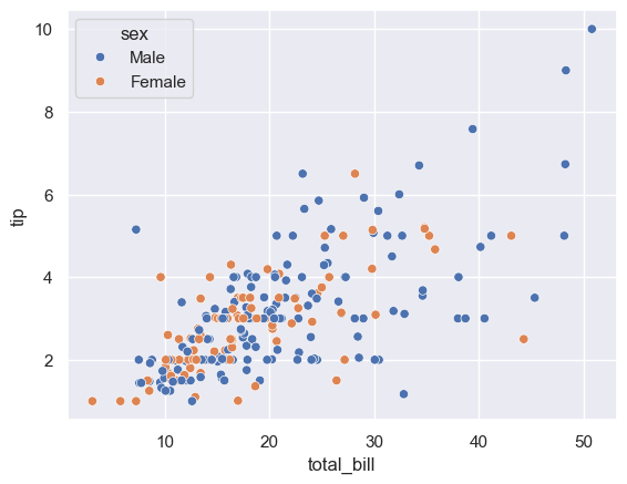
sns.scatterplot(data=tips, x="total_bill", y="tip", hue="day")<Axes: xlabel='total_bill', ylabel='tip'>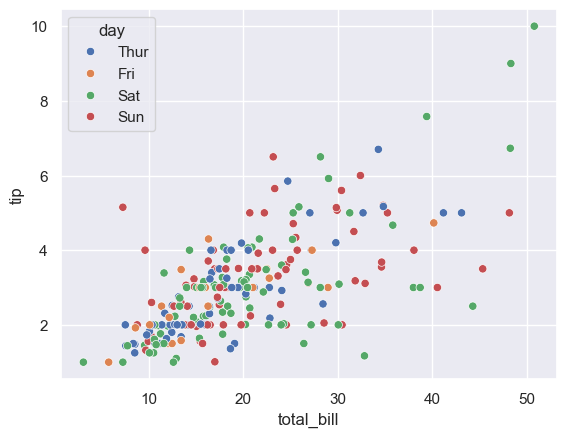
sns.scatterplot(data=tips, x="total_bill", y="tip", hue="sex", style="time")<Axes: xlabel='total_bill', ylabel='tip'>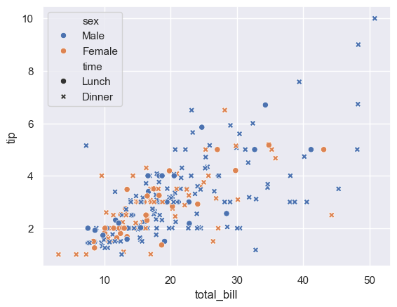
sns.scatterplot(data=tips, x="total_bill", y="tip", hue="sex", style="sex")<Axes: xlabel='total_bill', ylabel='tip'>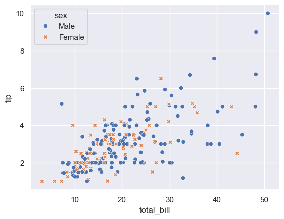
sns.scatterplot(data=tips, x="total_bill", y="tip", size="size")<Axes: xlabel='total_bill', ylabel='tip'>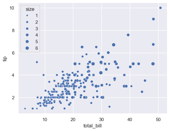
sns.scatterplot(data=tips, x="total_bill", y="tip", size="size", hue="sex")<Axes: xlabel='total_bill', ylabel='tip'>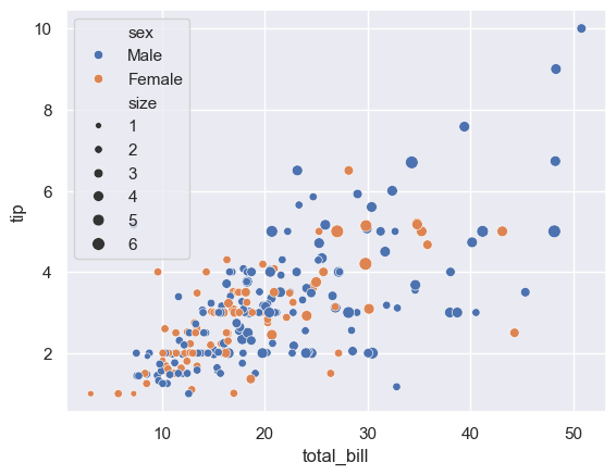
Seaborn Line Plots
flights = sns.load_dataset("flights")sns.lineplot(data=flights, x="year", y="passengers")<Axes: xlabel='year', ylabel='passengers'>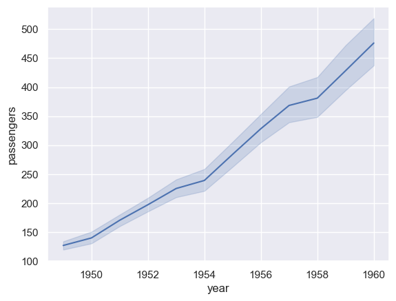
flights.groupby("year")["passengers"].mean().plot()<Axes: xlabel='year'>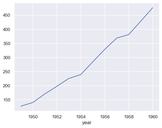
sns.lineplot(data=flights, x="year", y="passengers", estimator="sum")<Axes: xlabel='year', ylabel='passengers'>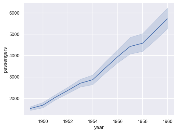
sns.lineplot(data=flights, x="year", y="passengers", hue="month")<Axes: xlabel='year', ylabel='passengers'>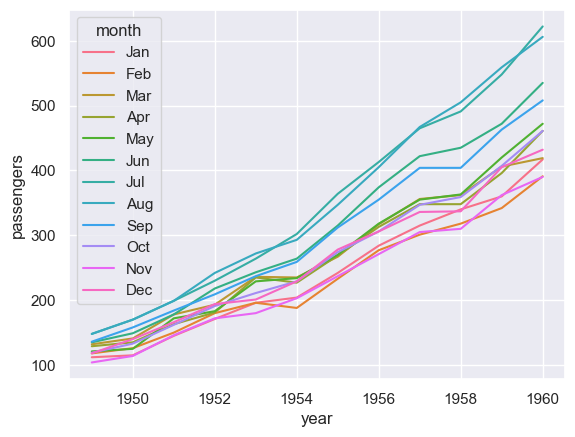
trips= sns.load_dataset("taxis", parse_dates=["pickup", "dropoff"])trips["hour"] = trips["pickup"].dt.hourtripsLoading...
sns.lineplot(data=trips, x="hour", y="total", hue="payment", style="color", ci=None)/tmp/ipykernel_51313/3291997563.py:1: FutureWarning:
The `ci` parameter is deprecated. Use `errorbar=None` for the same effect.
sns.lineplot(data=trips, x="hour", y="total", hue="payment", style="color", ci=None)
<Axes: xlabel='hour', ylabel='total'>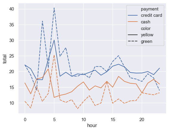
The Figure-Level Relplot( ) Method
tipsLoading...
sns.relplot(data=tips, x="total_bill", y="tip", kind="scatter", col="sex")<seaborn.axisgrid.FacetGrid at 0x7fd9209eda90>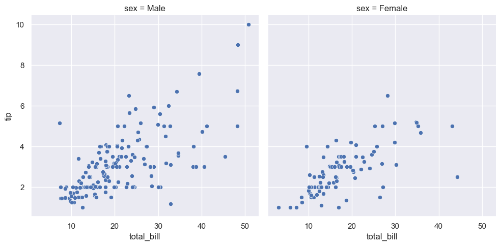
sns.relplot(data=tips, x="total_bill", y="tip", kind="scatter", hue="smoker", col="sex")<seaborn.axisgrid.FacetGrid at 0x7fd91e772c10>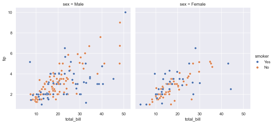
sns.relplot(data=tips, x="total_bill", y="tip", kind="scatter", hue="smoker", col="sex", row="time")<seaborn.axisgrid.FacetGrid at 0x7fd91e4942d0>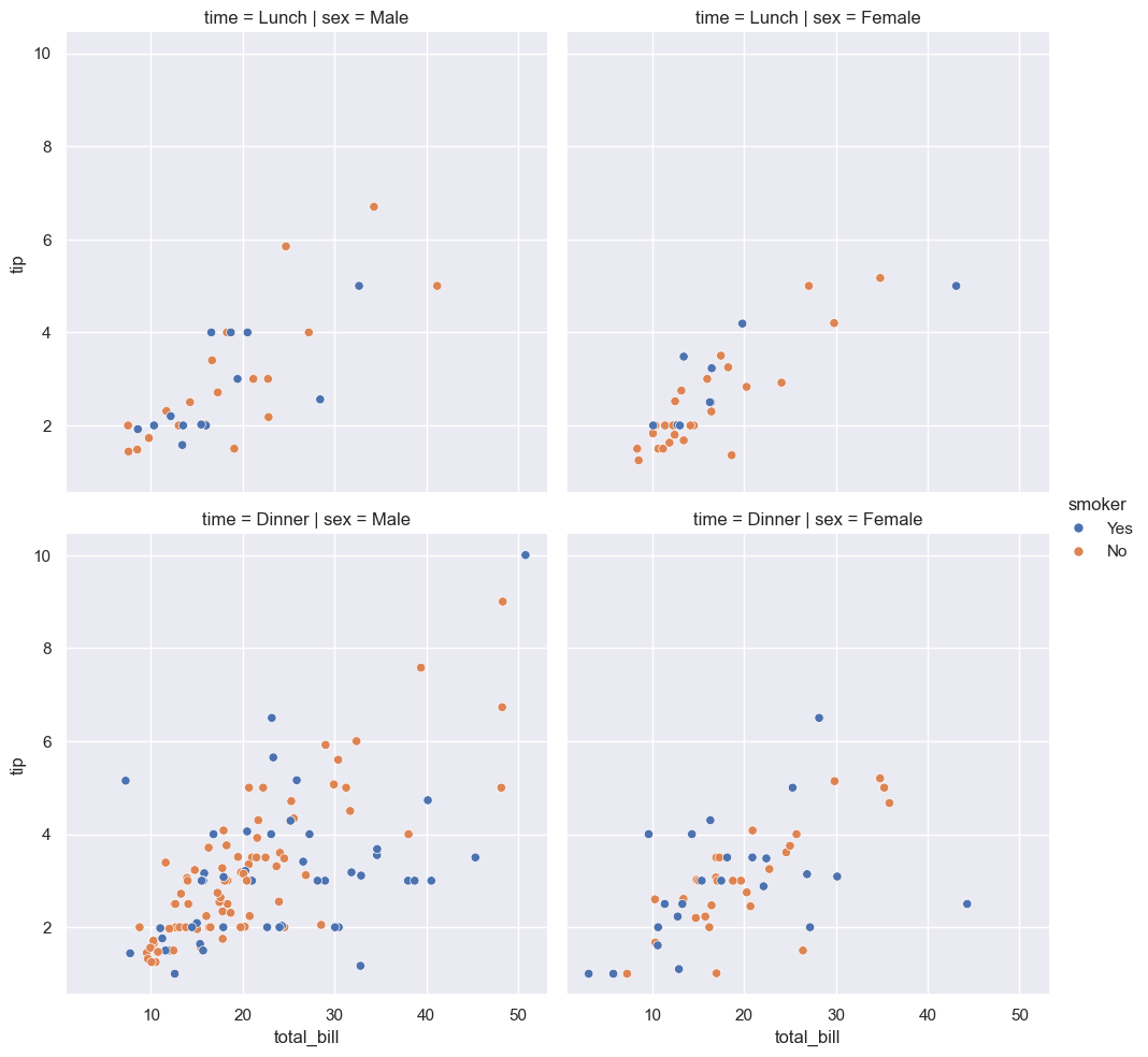
sns.relplot(data=trips, x="hour", y="total", kind="line", col="pickup_borough", hue="payment")<seaborn.axisgrid.FacetGrid at 0x7fd91e432350>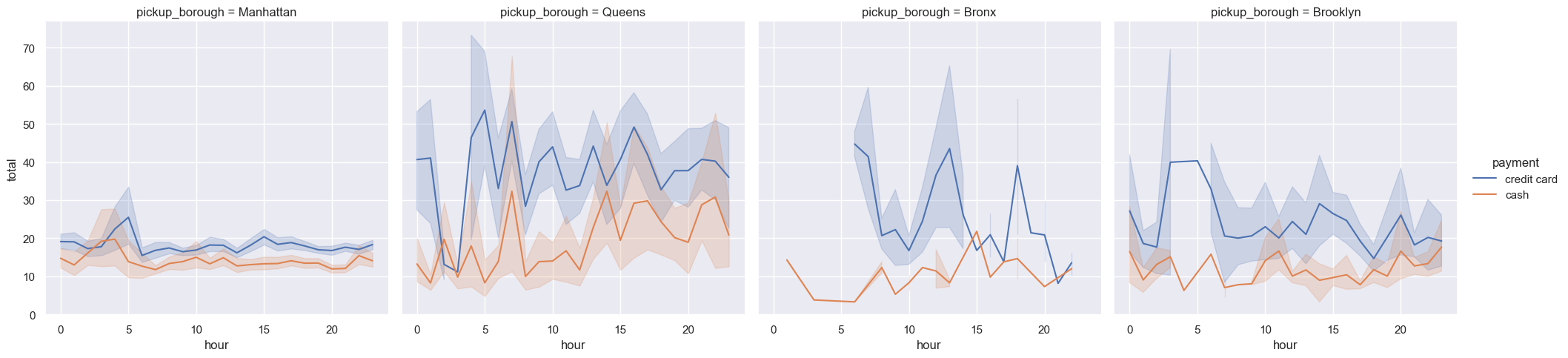
sns.relplot(
    data=trips,
    x="hour",
    y="total",
    kind="line",
    col="pickup_borough",
    hue="payment",
    row="dropoff_borough"
)
<seaborn.axisgrid.FacetGrid at 0x7fd91e047110>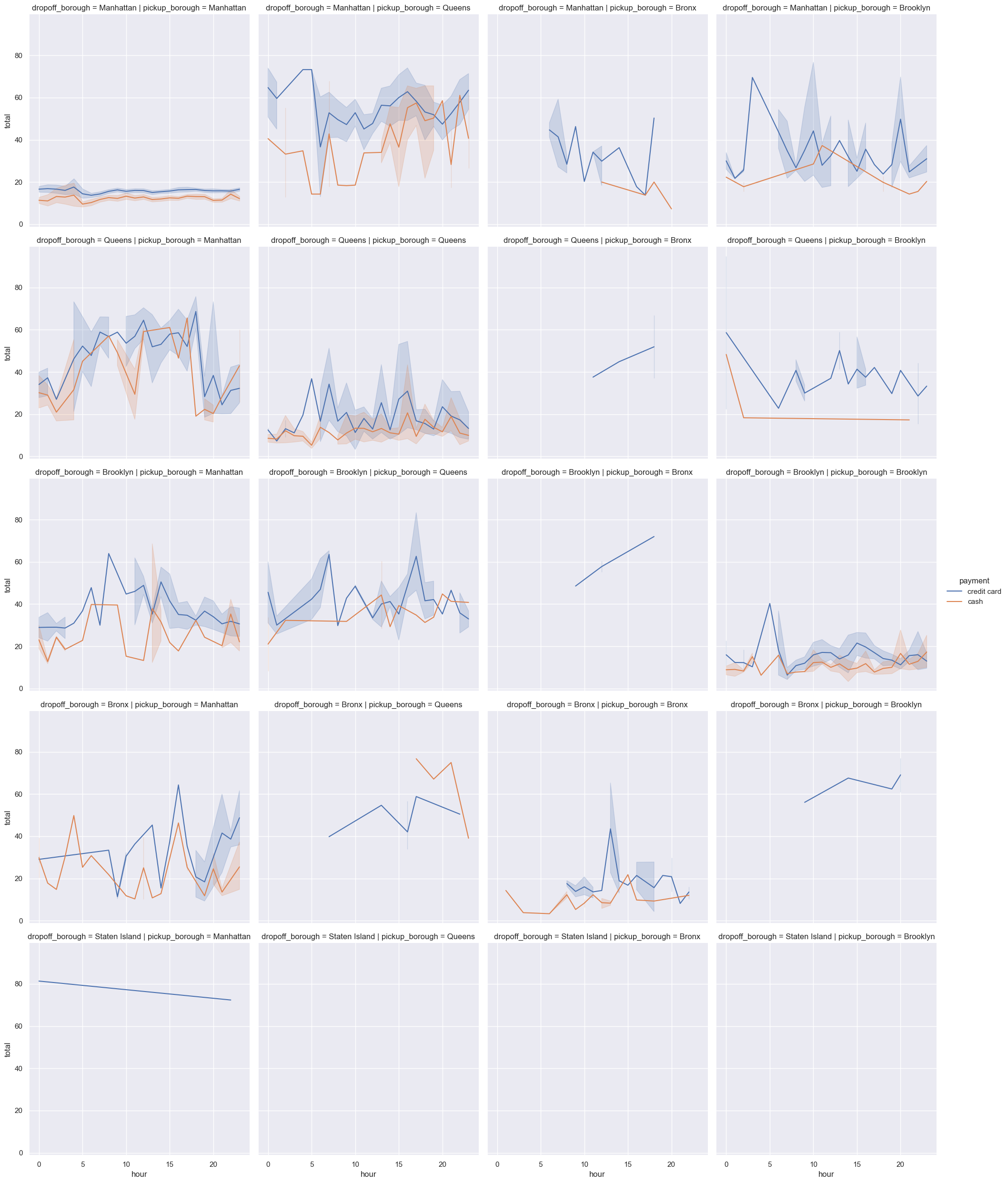
Changing Plot Sizes
plt.figure(figsize=(8,5))
sns.lineplot(data=flights, x="year", y="passengers", hue="month")
<Axes: xlabel='year', ylabel='passengers'>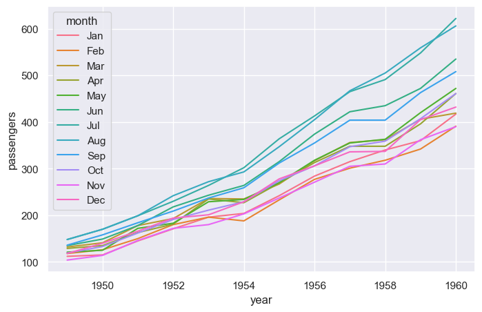
sns.relplot(
    data=tips,
    x="total_bill",
    y="tip",
    kind="scatter",
    hue="smoker",
    col="day",
    row="sex",
    height=2,
    aspect=2
)
<seaborn.axisgrid.FacetGrid at 0x7fd91cc7afd0>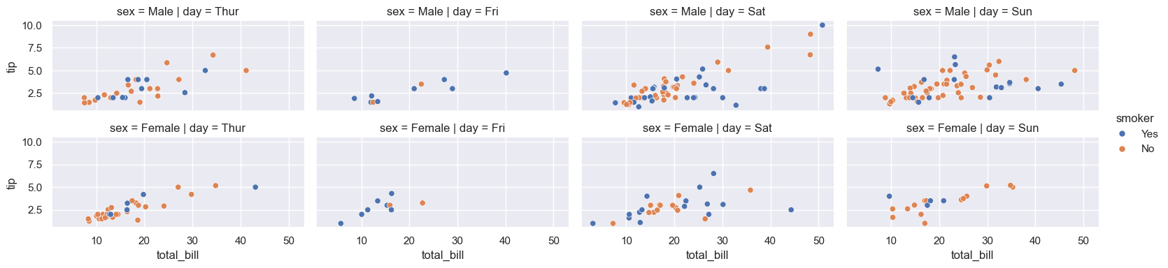
Seaborn Histograms
sns.histplot(data=tips, x="tip")<Axes: xlabel='tip', ylabel='Count'>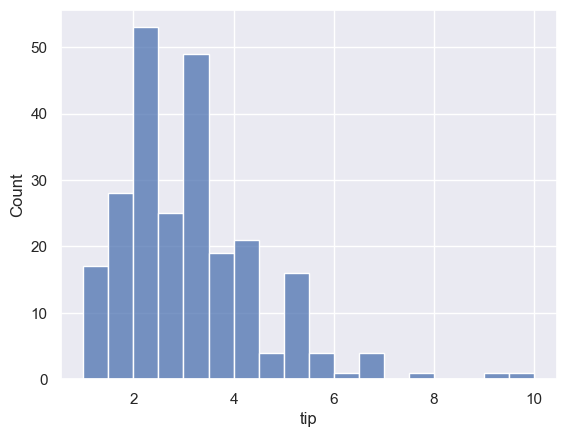
sns.histplot(data=tips, x="tip", hue="time")<Axes: xlabel='tip', ylabel='Count'>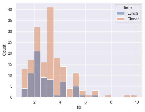
sns.histplot(data=tips, x="tip", hue="smoker", multiple="stack")<Axes: xlabel='tip', ylabel='Count'>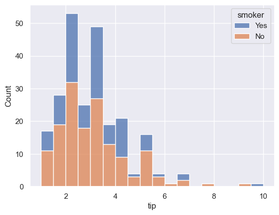
sns.histplot(data=tips, x="tip", hue="smoker", multiple="dodge")<Axes: xlabel='tip', ylabel='Count'>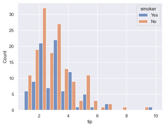
sns.histplot(data=penguins, x="body_mass_g", binwidth=500)<Axes: xlabel='body_mass_g', ylabel='Count'>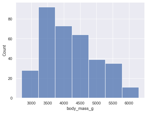
sns.histplot(data=penguins, x="body_mass_g", bins=20)<Axes: xlabel='body_mass_g', ylabel='Count'>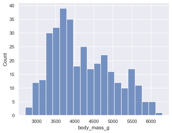
sns.histplot(data=penguins, x="body_mass_g", bins=20, hue="species", multiple="stack")<Axes: xlabel='body_mass_g', ylabel='Count'>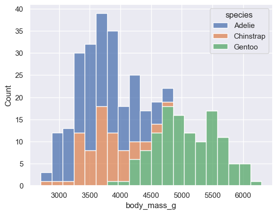
sns.histplot(data=penguins, x="body_mass_g", bins=20, hue="species", multiple="stack", element="step")<Axes: xlabel='body_mass_g', ylabel='Count'>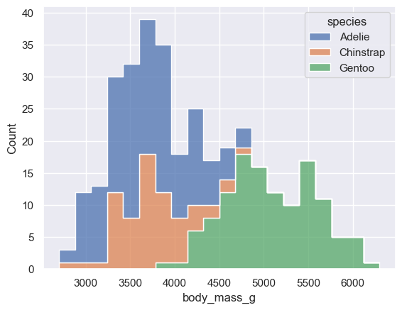
sns.histplot(data=tips, x="tip", kde=True)<Axes: xlabel='tip', ylabel='Count'>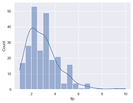
sns.set_theme()
plt.figure(dpi=200)
sns.histplot(
    data=penguins,
    x="body_mass_g",
    hue="species",
    multiple="stack",
    palette="muted",
    bins=20,
    kde=True
)
plt.title("Penguin Body Mass")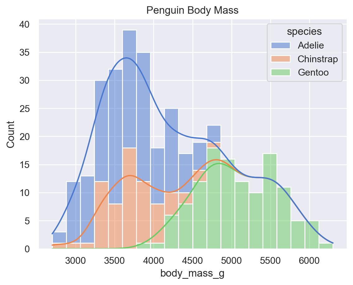
sns.set_theme()
plt.figure(dpi=200)
sns.histplot(
    data=penguins,
    x="body_mass_g",
    bins=20,
    hue="species",
    multiple="stack",
    kde=True
)
plt.title("Penguin Body Mass")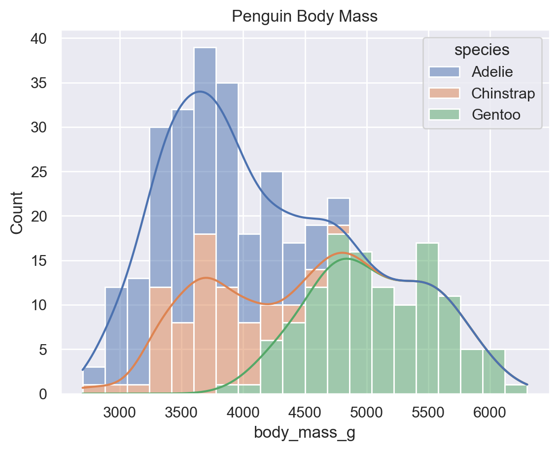
Seaborn KDE Plots
sns.kdeplot(data=penguins, x="body_mass_g")<Axes: xlabel='body_mass_g', ylabel='Density'>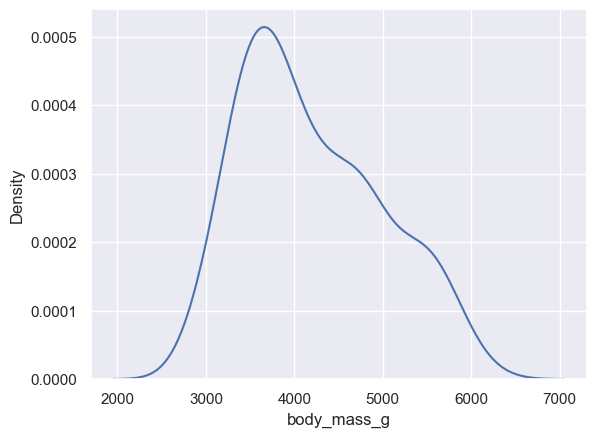
sns.kdeplot(data=penguins, x="body_mass_g", hue="species")<Axes: xlabel='body_mass_g', ylabel='Density'>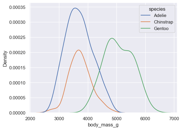
sns.kdeplot(data=penguins, x="body_mass_g", hue="species", bw_adjust=0.4)<Axes: xlabel='body_mass_g', ylabel='Density'>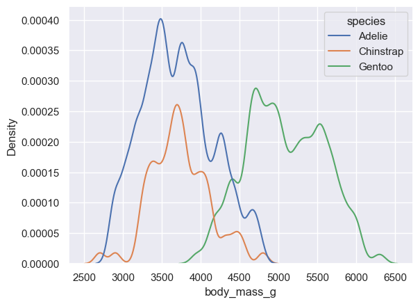
sns.kdeplot(data=penguins, x="body_mass_g", hue="species", multiple="stack")<Axes: xlabel='body_mass_g', ylabel='Density'>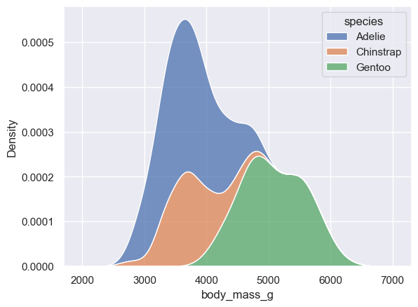
penguinsLoading...
sns.histplot(data=penguins, x="flipper_length_mm")<Axes: xlabel='flipper_length_mm', ylabel='Count'>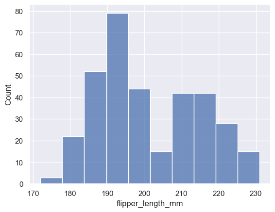
sns.histplot(data=penguins, x="body_mass_g")<Axes: xlabel='body_mass_g', ylabel='Count'>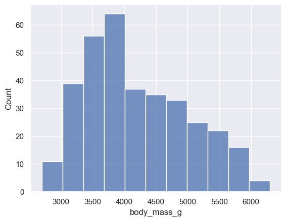
sns.histplot(data=penguins, x="body_mass_g", y="flipper_length_mm")<Axes: xlabel='body_mass_g', ylabel='flipper_length_mm'>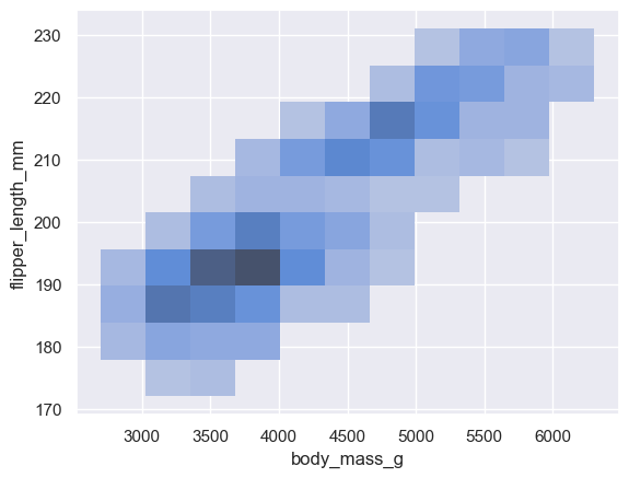
sns.kdeplot(data=penguins, x="body_mass_g", y="flipper_length_mm")<Axes: xlabel='body_mass_g', ylabel='flipper_length_mm'>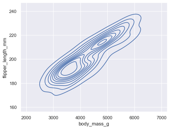
sns.kdeplot(data=penguins, x="bill_length_mm", y="flipper_length_mm", hue="species")<Axes: xlabel='bill_length_mm', ylabel='flipper_length_mm'>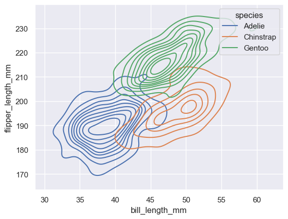
sns.histplot(data=penguins, x="bill_length_mm", y="flipper_length_mm", hue="species")<Axes: xlabel='bill_length_mm', ylabel='flipper_length_mm'>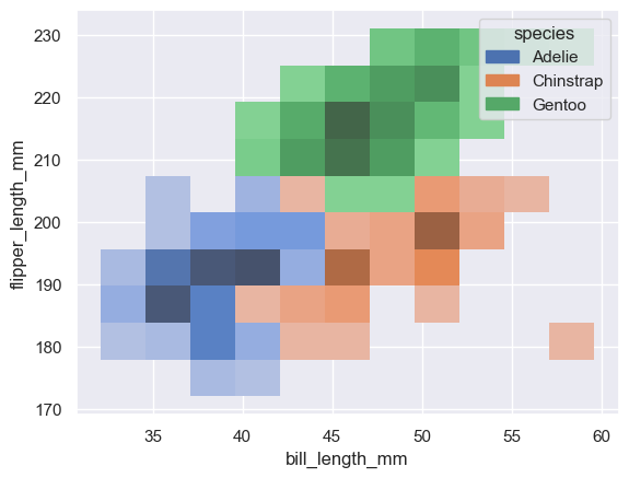
Seaborn Rugplots
sns.rugplot(data=tips, x="tip", height=0.2)<Axes: xlabel='tip'>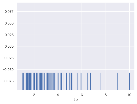
sns.rugplot(data=tips, y="tip", height=0.2)<Axes: ylabel='tip'>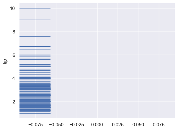
sns.kdeplot(data=tips, x="total_bill")
sns.rugplot(data=tips, x="total_bill", height=0.07)
<Axes: xlabel='total_bill', ylabel='Density'>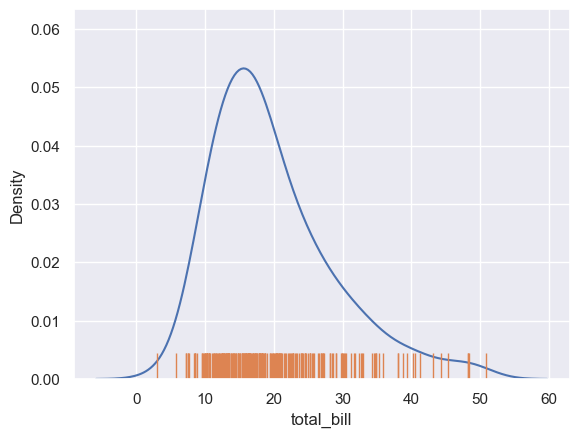
sns.scatterplot(data=tips, x="total_bill", y="tip")
sns.rugplot(data=tips,x="total_bill", y="tip")
<Axes: xlabel='total_bill', ylabel='tip'>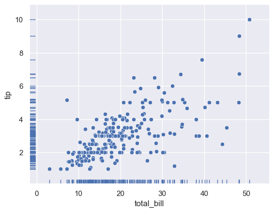
diamonds = sns.load_dataset("diamonds")
sns.scatterplot(data=diamonds, x="carat", y="price", s=5)
sns.rugplot(data=diamonds, x="carat", y="price", lw=1, alpha=.005)
<Axes: xlabel='carat', ylabel='price'>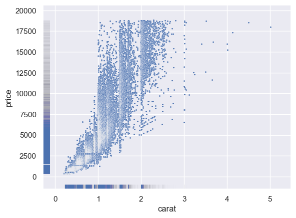
The Figure-Level hisplot( ) Method
sns.displot(kind="hist", data=penguins, x="body_mass_g", height=3, aspect=2)<seaborn.axisgrid.FacetGrid at 0x7fd915d7d6d0>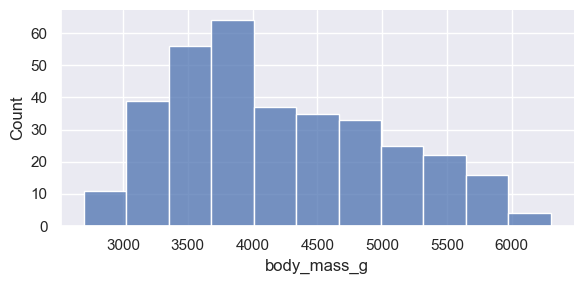
sns.displot(
    kind="hist",
    data=penguins,
    hue="sex",
    x="body_mass_g",
    col="species"
)
<seaborn.axisgrid.FacetGrid at 0x7fd91015c190>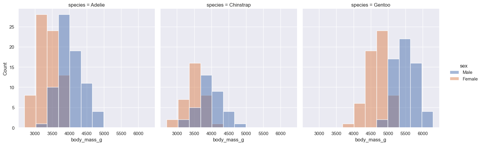
sns.displot(data=tips, kind="kde", x="tip", col="time", rug=True)<seaborn.axisgrid.FacetGrid at 0x7fd90be32c10>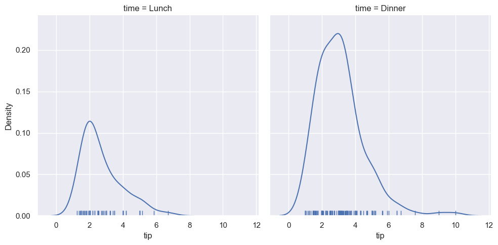
sns.displot(data=tips, kind="kde", x="total_bill", y="tip", rug=True)<seaborn.axisgrid.FacetGrid at 0x7fd90bd3ead0>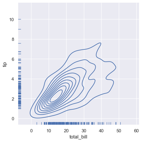
Seaborn Countplots
sns.countplot(data=penguins, x="species")<Axes: xlabel='species', ylabel='count'>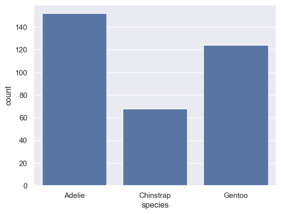
sns.countplot(data=penguins, x="species", hue="sex")<Axes: xlabel='species', ylabel='count'>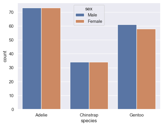
titanic = pd.read_csv("data/titanic.csv")sns.countplot(data=titanic, x="pclass", hue="sex")<Axes: xlabel='pclass', ylabel='count'>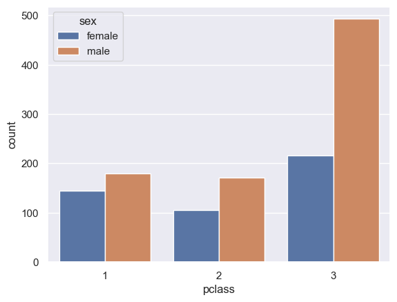
sns.countplot(data=titanic, y="pclass", hue="sex")<Axes: xlabel='count', ylabel='pclass'>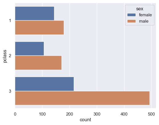
Seaborn Stripplot & Swarmplot
sns.scatterplot(data=trips, x="pickup_borough", y="distance")<Axes: xlabel='pickup_borough', ylabel='distance'>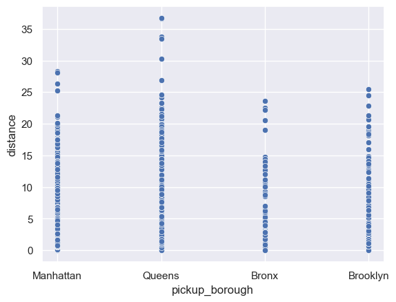
plt.figure(dpi=100)
sns.stripplot(data=trips, x="pickup_borough", y="distance")
plt.title("Taxi Trip Distance By Burough")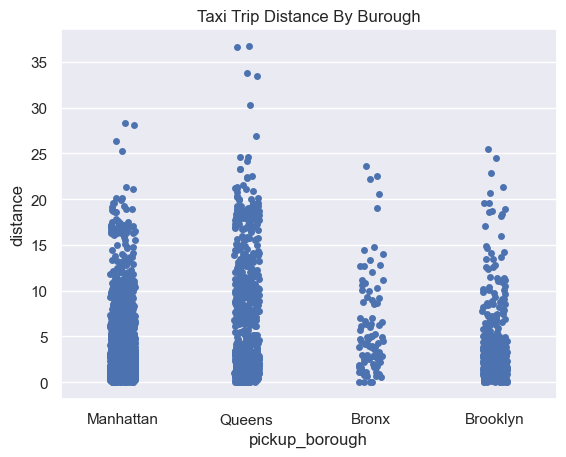
trips_sample = trips.nlargest(600, "total")plt.figure(figsize=(12,5))
sns.swarmplot(data=trips_sample, x="pickup_borough", y="distance")<Axes: xlabel='pickup_borough', ylabel='distance'>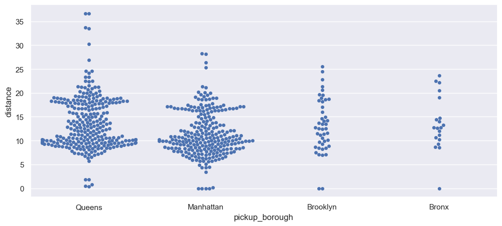
plt.figure(figsize=(12,5))
sns.stripplot(data=trips_sample, x="pickup_borough", y="distance")
plt.title("Taxi Trips By Borough")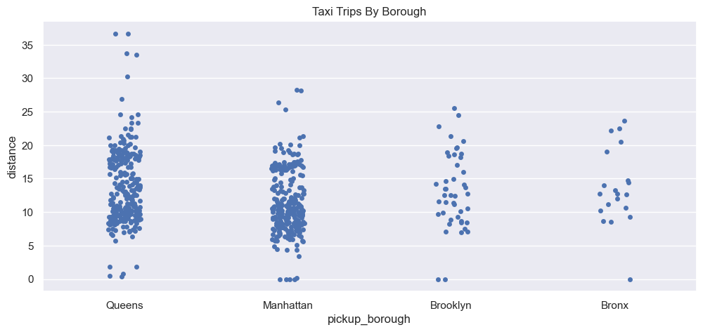
titanic = sns.load_dataset("titanic")plt.figure(figsize=(12,5))
sns.swarmplot(data=titanic, x="pclass", y="age", hue="sex")<Axes: xlabel='pclass', ylabel='age'>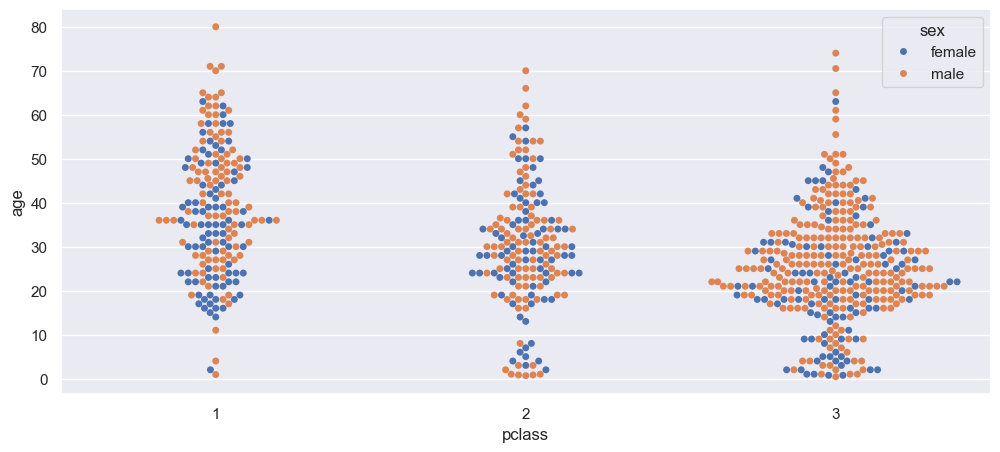
Seaborn Boxplots
sns.boxplot(data=titanic, x="age")<Axes: xlabel='age'>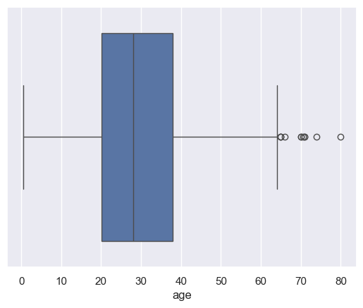
sns.boxplot(data=trips, x="pickup_borough", y="total")<Axes: xlabel='pickup_borough', ylabel='total'>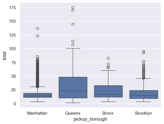
sns.boxplot(data=trips, x="pickup_borough", y="total", whis=2.5, fliersize=2)<Axes: xlabel='pickup_borough', ylabel='total'>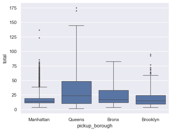
sns.boxplot(data=titanic, x="pclass", y="age", hue="sex", fliersize=5)<Axes: xlabel='pclass', ylabel='age'>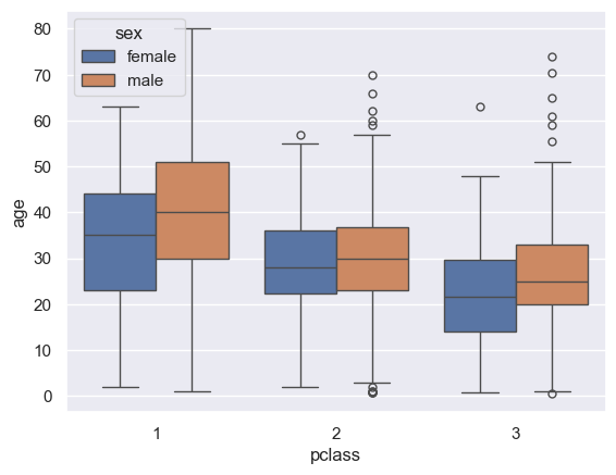
sns.boxplot(data=penguins, x="species", y="body_mass_g")
sns.swarmplot(data=penguins, x="species", y="body_mass_g", color="0.3")
<Axes: xlabel='species', ylabel='body_mass_g'>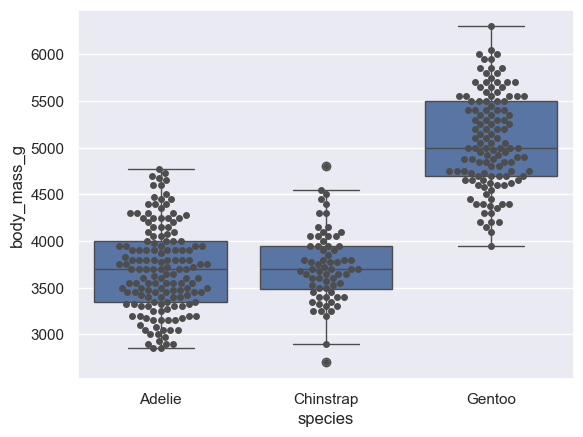
Seaborn Boxenplots
sns.boxplot(data=trips, x="pickup_borough", y="total")<Axes: xlabel='pickup_borough', ylabel='total'>plt.figure(figsize=(10,6))
sns.boxenplot(data=trips, x="pickup_borough", y="total")<Axes: xlabel='pickup_borough', ylabel='total'>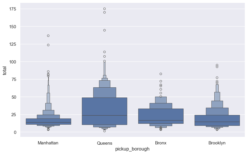
Seaborn Violinplots
sns.violinplot(data=titanic, x="age")
# sns.boxplot(data=titanic, x="age")
<Axes: xlabel='age'>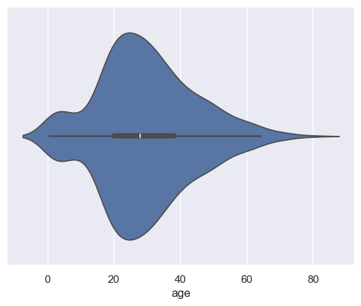
sns.violinplot(data=titanic, x="pclass", y="age")<Axes: xlabel='pclass', ylabel='age'>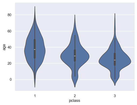
sns.violinplot(data=titanic, x="pclass", y="age", hue="sex")<Axes: xlabel='pclass', ylabel='age'>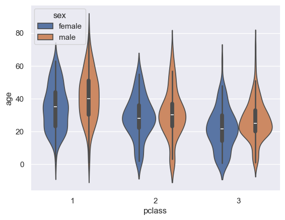
plt.figure(figsize=(10,4))
sns.violinplot(data=titanic, x="pclass", y="age", hue="sex", split=True, palette="muted")
<Axes: xlabel='pclass', ylabel='age'>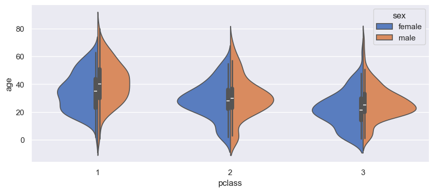
Seaborn Barplots
sns.barplot(data=trips, x="pickup_borough", y="distance")<Axes: xlabel='pickup_borough', ylabel='distance'>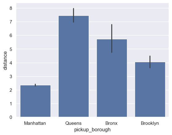
sns.barplot(data=trips, x="pickup_borough", y="total")<Axes: xlabel='pickup_borough', ylabel='total'>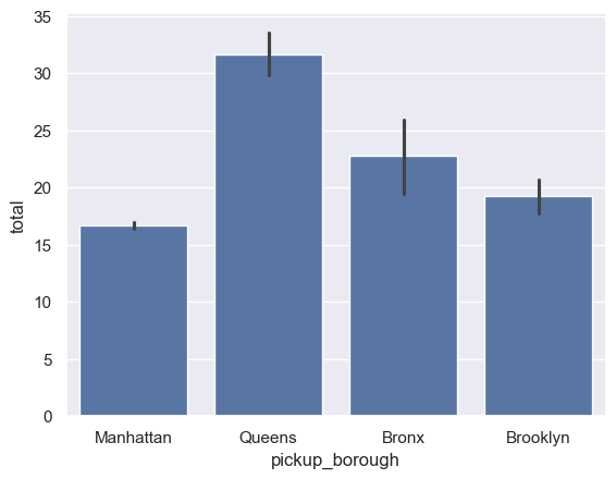
sns.barplot(data=trips, x="pickup_borough", y="total", estimator=sum)<Axes: xlabel='pickup_borough', ylabel='total'>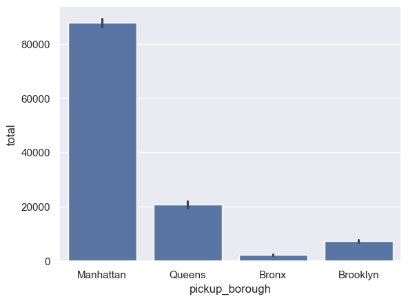
trips.groupby("pickup_borough")["total"].sum().plot(kind="bar")<Axes: xlabel='pickup_borough'>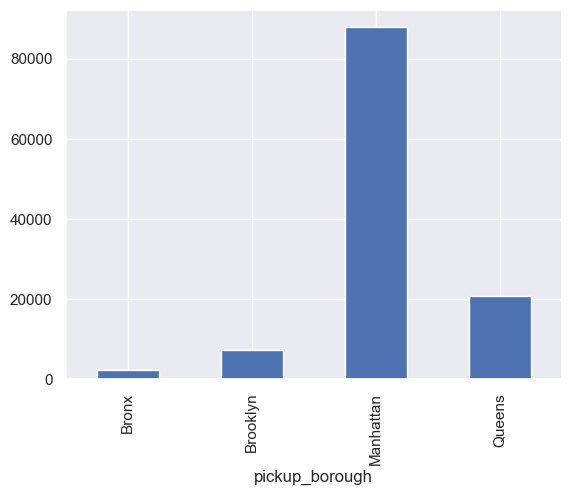
sns.barplot(data=trips, x="pickup_borough", y="distance", hue="color")<Axes: xlabel='pickup_borough', ylabel='distance'>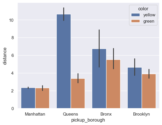
sns.barplot(data=trips, y="pickup_borough", x="distance", hue="color", dodge=False)<Axes: xlabel='distance', ylabel='pickup_borough'>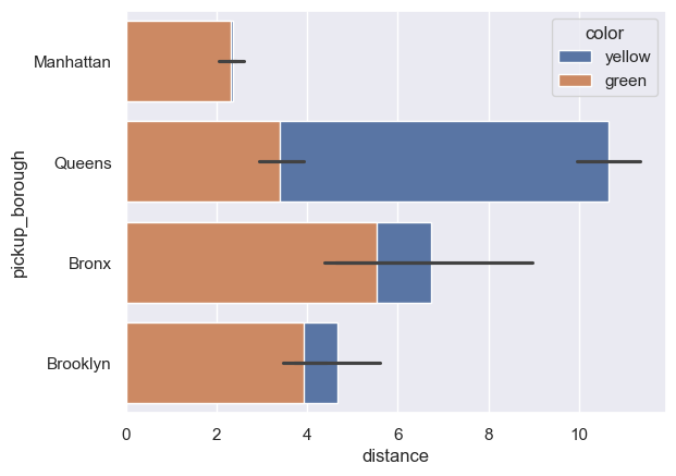
sns.barplot(data=titanic, y="pclass", x="survived", orient="h")<Axes: xlabel='survived', ylabel='pclass'>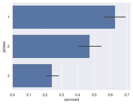
The Figure-Level catplot( ) Method
sns.catplot(data=titanic, x="sex", y="survived", kind="bar")<seaborn.axisgrid.FacetGrid at 0x7fd90afe3390>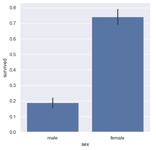
sns.catplot(data=titanic, x="sex", y="survived", kind="bar", col="pclass")<seaborn.axisgrid.FacetGrid at 0x7fd90ae656d0>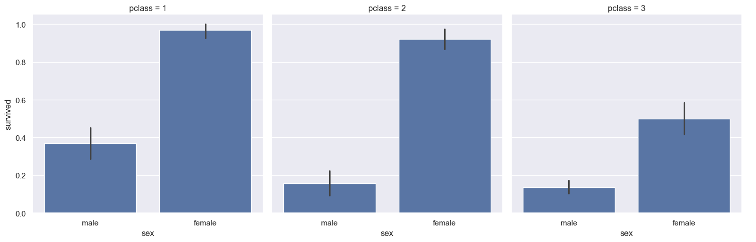
sns.catplot(data=titanic, x="pclass", y="survived", kind="bar", hue="sex")<seaborn.axisgrid.FacetGrid at 0x7fd90ad7bc50>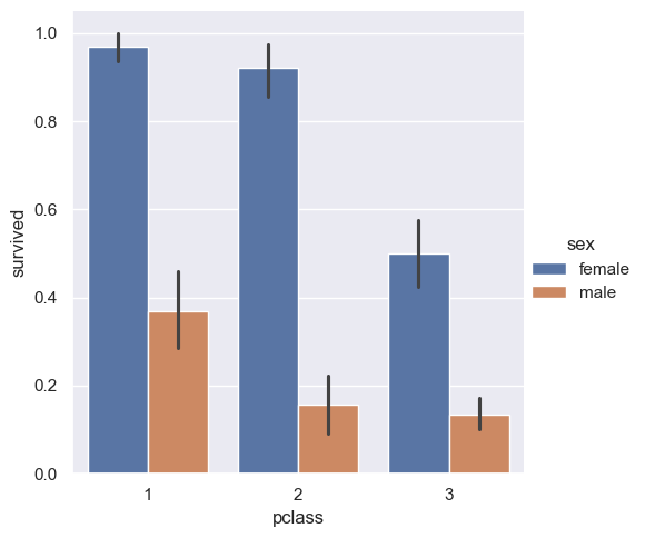
sns.catplot(
    data=trips,
    kind="strip",
    x="pickup_borough",
    y="distance",
    col="color",
    aspect=0.8
)
<seaborn.axisgrid.FacetGrid at 0x7fd90ac0b250>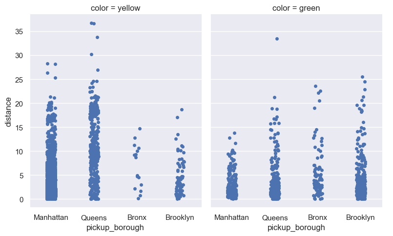
sns.catplot(data=trips, kind="violin", x="pickup_borough", y="distance", hue="color", split=True)<seaborn.axisgrid.FacetGrid at 0x7fd90ab134d0>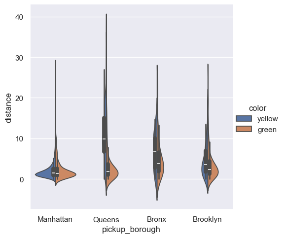
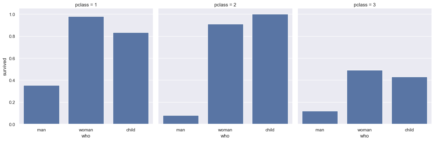
sns.catplot(
    data=titanic,
    kind="bar",
    x="who",
    y="survived",
    col="pclass",
    ci=None,
)
/tmp/ipykernel_51313/1873499506.py:1: FutureWarning:
The `ci` parameter is deprecated. Use `errorbar=None` for the same effect.
sns.catplot(
<seaborn.axisgrid.FacetGrid at 0x7fd90abf4550>